A map of the Pacific

The projection is “+proj=lee_os +ellps=GRS80”

And yes, the GMT coastlines would be absolutely fine (though I did notice differences between the GMT and OpenStreetMap pushing the 500 m mark in some places). But I just felt like using the OpenStreetMap.

I’ve accidentally deleted the -R - for real. But this is what I did. I looked at the 1974 map, and did a gmt mapproject for the corners of the map to get the region in projected metres. When I’ve recovered the script I’ll post it here.

Edit: this is a bit bigger than the original 1974 map: -R-10291000/11278000/-8219000/9039000 It’s what I’m using when projecting the topography.

But for the topography you are projecting the xyz and later grid them, right?

And, BTW, I have started a Weather Maps category in the GMT.jl docs. Please feel free to add more from your collection.The current Windbarbs example looks artistic but it was not on purpose. Apparently the region alias for R was not implemented.

1 Like

That’s what I was thinking. I’m currently downloading the hundreds of geotiffs from Japan, and converting them to 1 arc second resolution tiles. The Japanese DEM site doesn’t seem to let me download the whole world in one go - I am literally clicking on hundreds of links …

After that I’ll probably reduce the resolution to 15 or 30 arc seconds and project them onto the oblated stereographic grid.

The Copernicus GDEM30 is probably a better dataset (have a recall that ALOS was not particularly good) OpenTopography - Copernicus Global Digital Elevation Models
lets you download programmatically (with curl).

1 Like

Oh dear. I sense a massive rabbit hole :grinning_face:. A quick search found Copernicus is highly regarded: A performance comparison of SRTM v. 3.0, AW3D30, ASTER GDEM3, Copernicus and TanDEM-X for tectonogeomorphic analysis in the South American Andes - ScienceDirect

But for a global map, they’re probably all fine. I should have stuck with SRTM for ease of use!

Going down the DEM rabbit hole. There are at least three free DEMs: Copernicus, ALOS and SRTM.

One thing we used to do with gridded weather forecasts is something called a poor man’s ensemble - basically average gridded weather forecasts from different centres. The average forecast usually performed better on scores such as root mean square error than any individual forecast. It’s quite likely an average of the DEMs would be closer to the “truth” than any single DEM. It would be smoother - which may or may not be a good thing, depending on what the user wants.

To be proved but I doubt it. There are more than 20 years between SRTM and TandemX. GDT30 is a downsampled version of the oirinal 12m TandemX.

I noticed that the ALOS DEM qualitatively looked to be more accurate than SRTM in the Tonga region. I saw ALOS resolve small islands that SRTM missed. But in the middle of the land, I couldn’t say whether one or the other DEM was closer to whatever the truth is. I know there are LIDAR data for at least the main island of Tonga which could be taken as a “truth” dataset (they’ve discovered interesting archaeological features from these data - despite archaeology not being the main reason for collecting the data). Unfortunately, the data don’t appear to be in the public domain.

Regarding the difference between the C/C++ calculations in PROJ differing from the little piece of Julia code. It’s quite likely PROJ and the Julia are using different math libraries - Julia uses something called openlibm I think. One of the guys at work found the actual code for the trigonometric functions used in gcc/g++. They all claim to be exact to the last bit of floating point, but there is no guarantee the two libraries produce the exact same results. To do any projection from (lon, lat) to (x, y) there are quite a few trigonometric functions called, plus a number of multiplications, divisions and so on. We couldn’t say if it was just accumulating roundoff errors or not, but it didn’t seem an implausible explanation.

Another explanation is that the underlying equations in PROJ may be different. This issue crops up in spherical geometry a bit - see this page for more information: Great-circle distance - Wikipedia. The simplest formula for distances between points on a sphere is not accurate (because of numerical precision issues) when the points are close together. But there are other equations that avoid this and produce accurate distances even for close together points.

I would lean more to the second alternative. Although the math libs are different the guys in Julia are absolutely paranoiac with precision to the last bit, most accurate algorithms to do summations (where order actually matters), etc.

1 Like

I was contemplating running the calculations in quadruple precision. But then sanity returned, and if I don’t care about 500 m differences (being below the resolution of the pixels in my map), I certainly don’t care about sub-metre differences!

Experimentation so far. I gave up on the newer DEMs because they were taking way too long to process, and instead fell back to the old SRTM DEM because it’s easy to use. pacific_500m.gmt is a simplified coastline from OpenStreetMap. I’m not sure if the projection of the SRTM data is being done properly - I’m still learning about gmt surface etc. But the end map is starting to look nice.

#!/usr/bin/env bash

proj="+proj=lee_os +ellps=GRS80"
proj_region="-R-10674773/10691707/-8028940/8499687"
geog_region="-R70/330/-90/80"

#gmt mapproject pacific_500m.gmt -J"${proj}" ${geog_region} -bi2f -bo2f > coast.gmt
#gmt grdcut @earth_relief_30s ${geog_region} -Gtopo.nc
#gmt grd2xyz topo.nc | gmt mapproject -J"${proj}" ${geog_region} -bo3f | \
#	gmt blockmean -I1000/1000 -R-10675000/10692000/-8029000/8500000 -bi3f -bo3f | \
#	gmt surface -I1000/1000 -R-10675000/10692000/-8029000/8500000 -Gpactopo.nc -bi3f

gmt begin pacific png
	gmt makecpt -Cetopo1 -T-6000/5000/250
	gmt grdimage pactopo.nc -Jx1:50000000 ${proj_region} -I
	gmt plot coast.gmt -Wfaint,black -bi2f
gmt end

3 Likes

Yes, looks nice though the illumination could look nicer. Try without the gmt makecpt -Cetopo1 -T-6000/5000/250 (let the automatic thing do its work).
The big drawback of this type of approach is that we’ll have no frames or annotations and even a grid is a bit problematic.

I totally agree that frames, annotations and grids are a problem. But one has to make use of what is available :slight_smile: I have an idea for adding them all, without that much difficulty, I just haven’t got around to it yet.

Is the grd2xyz | blockmean | surface thing roughly about right? surface still complained even though I used blockmean. And that took all night to process on my little Mac mini. These DEMs sure do require a lot of grunt to manipulate!

surface is very heavy. You can have an indistinguishable figure at this scale if you use nearneighbor

Eager to see your frames/annots idea.

And it would also worth trying gdalwarp

1 Like

This is the most hideous bash script in the world below. It annotates the frames and draws grid lines on the Oblated Stereographic map of the Pacific. It really would be better in a language like Julia. But it works.

To get the annotations on the frame, I created lists of (Lon, lat) for the points along the edge, and then used gmt sample1d to interpolate to evenly spaced latitudes or longitudes. But the catch was gmt sample1d expects monotonically increasing or decreasing data. So I need to break the lists of latitudes and longitudes up into individual files where this monotonic requirement is met.

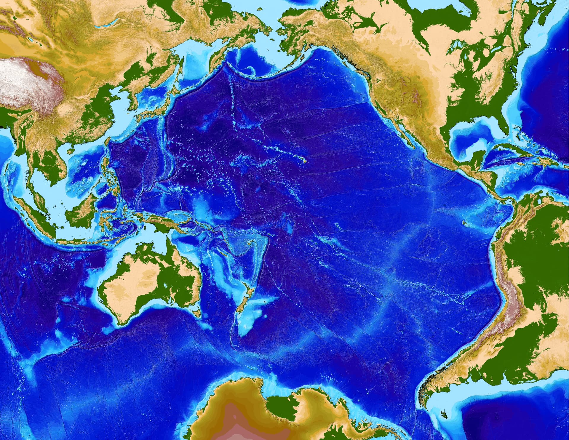
Unfortunately I cannot upload any images to the forum at the moment - is something broken? The map is starting to look quite nice.

#!/usr/bin/env bash

proj="+proj=lee_os +ellps=GRS80"
proj_region="-R-10674773/10691707/-8028940/8499687"
geog_region="-R70/330/-90/80"

function grid(){
	local spc="${2}"
	for lat in $(seq -80 10 80)
	do
		echo ">"
		gmt math -T70/330/1 ${lat} = | gmt mapproject -J"${proj}" ${geog_region}
	done
	for lon in $(seq 70 10 330)
	do
		echo ">"
		gmt math -o1,0 -T-90/80/1 ${lon} = | gmt mapproject -J"${proj}" ${geog_region}
	done
}

function monotonic(){
	local col="${1}"
	local spc="${2}"
	awk -v spc="${spc}" -v col="${col}" '
	{
		if (col == 3){
			val = ($col < 0) ? $col + 360 : $col;
		} else {
			val = $col;
		}
	}
	NR==1{
		file_num = 1;
		file=sprintf("labels_%04d.txt", file_num)
		printf("%f\t%f\t%f\n", $1, $2, val) > file;
		prev_val = val;
	}
	NR==2{
		incdec = val-prev_val;
		printf("%f\t%f\t%f\n", $1, $2, val) > file;
		prev_val = val;
	}
	NR>2{
		if (((val <= prev_val)&&(incdec < 0)) || ((val >= prev_val) && (incdec >= 0))){
			printf("%f\t%f\t%f\n", $1, $2, val) > file;
			prev_val = val
		} else {
			file_num++;
			file=sprintf("labels_%04d.txt", file_num)
			incdec = val-prev_val;
			printf("%f\t%f\t%f\n", $1, $2, val) > file;
			prev_val = val;
		}
	}'
}

function frame(){
	local region=$1
	local edge=$2
	local ll=$3
	local spc=$4
	case "${edge}" in
		"west")
			local order="1,0"
			local min=$(echo "${region}" | cut -d "/" -f 3)
			local max=$(echo "${region}" | cut -d "/" -f 4)
			local border=$(echo "${region}" | cut -d "/" -f 1)
			;;
		"east")
			local order="1,0"
			local min=$(echo "${region}" | cut -d "/" -f 3)
			local max=$(echo "${region}" | cut -d "/" -f 4)
			local border=$(echo "${region}" | cut -d "/" -f 2)
			;;
		"south")
			local order="0,1"
			local min=$(echo "${region}" | cut -d "/" -f 1)
			local max=$(echo "${region}" | cut -d "/" -f 2)
			local border=$(echo "${region}" | cut -d "/" -f 3)
			;;
		"north")
			local order="0,1"
			local min=$(echo "${region}" | cut -d "/" -f 1)
			local max=$(echo "${region}" | cut -d "/" -f 2)
			local border=$(echo "${region}" | cut -d "/" -f 4)
			;;
	esac

	if [[ "${ll}" == "lon" ]]
	then
		local col=3;
	else
		local col=4;
	fi
	gmt math -o"${order}" -T${min}/${max}/10000 ${border} = label.xy
	gmt mapproject -I -J"${proj}" < label.xy > label.ll
	rm -f labels_????.txt
	paste label.xy label.ll | monotonic "${col}" "${spc}"
	ls -1 labels_????.txt | xargs -I file gmt sample1d file -N2 -T${spc} | awk \
		-v ll="${ll}" '
		{
			val=$3;
			if (ll == "lon"){
				if (val > 180){
					valstr=sprintf("%.f\260W", 360-val);
				} else {
					valstr=sprintf("%.f\260E", val);
				}
			} else {
				if (val < 0){
					valstr=sprintf("%.f\260S", -1*val);
				} else {
					valstr=sprintf("%.f\260N", val);
				}
			}
			printf("%f\t%f\t%s\n", $1, $2, valstr);
		}'
}

#gmt mapproject pacific_500m.gmt -J"${proj}" ${geog_region} -bi2f -bo2f > coast.gmt
#gmt grdcut @earth_relief_30s ${geog_region} -Gtopo.nc
#gmt grd2xyz topo.nc | gmt mapproject -J"${proj}" ${geog_region} -bo3f | \
#	gmt blockmean -I1000/1000 -R-10675000/10692000/-8029000/8500000 -bi3f -bo3f | \
#	gmt surface -I1000/1000 -R-10675000/10692000/-8029000/8500000 \
#	-Ll-11000 -Lu9000 -Gpactopo.nc -bi3f
#gmt grd2xyz topo.nc | gmt mapproject -J"${proj}" ${geog_region} -bo3f | \
#	gmt nearneighbor -I1000/1000 -R-10675000/10692000/-8029000/8500000 \
#		-S5000 -bi3f -Gpactopo.nc

gmt begin pacific PNG
	gmt grdimage pactopo.nc -Jx1:50000000 ${proj_region} -Cetopo1 -I
	gmt plot coast.gmt -Jx1:50000000 ${proj_region} -Wfaint,black -bi2f
	grid 10 | gmt plot -Wthinnest,white,.
	frame "-10675000/10692000/-8029000/8500000" "west" "lat" 10  | \
	gmt text -Jx1:50000000 ${proj_region} -F+a0+jLM+f8p,Helvetica,white \
		-N -Dj0.2c/0c
	frame "-10675000/10692000/-8029000/8500000" "north" "lon" 10  | \
	gmt text -Jx1:50000000 ${proj_region} -F+a90+jRM+f8p,Helvetica,white \
		-N -Dj0.2c/0c
	frame "-10675000/10692000/-8029000/8500000" "east" "lat" 10  | \
	gmt text -Jx1:50000000 ${proj_region} -F+a0+jRM+f8p,Helvetica,white \
		-N -Dj0.2c/0c

gmt end
1 Like

I am making this map for fun, to put on my wall as a poster. But a very real use would be for things like the tsunami yesterday from the big earthquake in Russia. All the maps I saw yesterday were on our old favourite, Mercator. Mercator stretches distances in the higher latitudes a lot more than the Oblated Stereographic. And tsunami travel times are of course directly related to distance from the earthquake. So moving away from something like Mercator has to be a good thing?

2 Likes

Tim, Tsunami Travel Times are computed directly in geographical coords.

I’m sure your map is nice but if we want reproducibility need to move it into GMT (or at least GMT.jl). Those bash scripts kill me just to sneak at them.

Of course tsunami travel times are computed correctly in the background. But all the warning maps I saw were Mercator. This makes Kamchatka look further away from the tropical regions than it really is. The final step of displaying data is important - even if the data themselves are good.

Yeah - I did warn that the scripts are the worst things in the world! I was hacking them together at high speed, and as I was doing them it occurred to me that some of the things I was doing would be much easier in almost any other language than shell script (except for the hurdle of having to learn said language!).

It doesn’t seem possible to upload images to the forum at the moment.