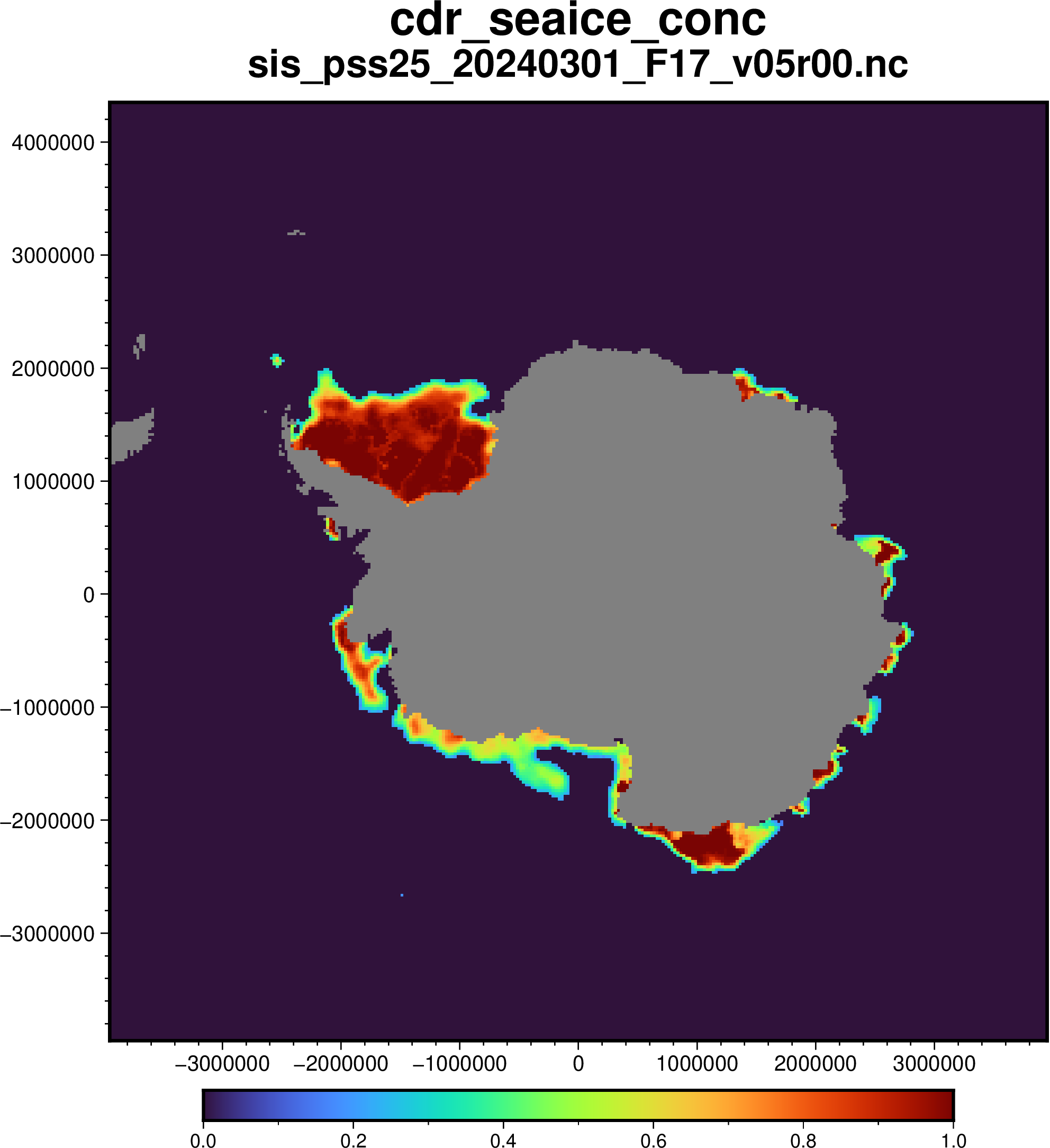
Sea-ice concentration in polar regions
Animation from Jan 2016 to Dec 2021

Movie built with The Generic Mapping Tools
Data
- Dataset available on Climate Data Store (CDS - Copernicus)
- Origin and sensor : EUMETSAT OSI SAF (coarse-resolution data from SMMR/SSMI/SSMIS)
- Type : ICDR (Interim Climate Data Record)
- Topography and bathymetry : GMT
@relief - Solar declination function from Hobbins et al. (2004), formula 16.
Runtime
Number of core used : 24
CPU Utilized: 00:12:29
Job Wall-clock time: 03:12:52
Memory Utilized: 3.39 GB
Pseudo-code
All figures are assigned an absolute position on an A4 paper (29.7 x 21 cm)
gmt begin canvas png
gmt basemap -R0/29.7/0/8 -JX29.7/8c -Bfg -B+gbisque
gmt basemap -R0/29.7/0/21 -JX29.7c/21c -Bafg
gmt end
NOTA : I initially used relative positionning between plots as well as the modern-mode inset module for the bottom part, but GMT doesn’t handle relative positions within inset, making the workaround unnecessarily illegible. cf github #6288 for those interested in GMT development.
The two main parts (upper panel) are stereographic projection (-Js) of the polar regions, centered on the poles. Their scale is manually choosen to fit the canvas restriction.
gmt mapproject -R0/360/65/90 -Js0/90/77/1:62200000 -Ww
Sea-Ice sheet
To plot the sea-ice concentration, I have to transform the NetCDF file from kilometers to degree in order to use grdimage. For smoother results, I also oversampled the data to fit the topography resolution I chose (grdsample)
gmt grdproject ${projection} ${region} ${data} -Gdata_bis.nc -C -I -Fk
gmt grdsample data_bis.nc+n0 -I1m -nl -Gdata_ter.nc
gmt grdimage data_ter.nc -Cice.cpt -Q ${projection} ${region} $posx $posy
Sea-Ice surface
Now that I have my ice sheet, I can roughly compute the sea-ice surface through time :
gmt grdmath data_bis.nc 1 GE AREA MUL SUM = tmp.nc
value=$(gmt grdinfo tmp.nc -T | awk -F[/] '{print $2}')
echo $day $value | gmt plot -Sc0.2c -Wthick,black -G${clor} $proj_vol $area_vol $posx_vol $posy_vol --FORMAT_DATE_IN=yyyymmdd
NOTA : The value obtained are not as precise as the one from the National Snow and Ice Data Center (NSIDC), but considering my approximation approach (grdmath line) and the data native resolution, the order of magnitude is decent.
Declination
Solar declination, i.e. the angle between the Earth’s rotation axis and the Solar equatorial plane, changes with the season as the former moves around the latter (let’s hope this is not too controversial). The angle is maximal at the solstices (June and December) and minimal at the equinoxes (March and September). The phenomenon is sufficiently similar from one year to another to use a “generic” year and loop it. To make it a notch fancier, I also threw a shading that tilts accordingly (-JG0/0/?c+w${delta}).
gmt math -foT --TIME_UNIT=d -T0/365/1 2 PI MUL T 1 SUB MUL 365 DIV STO@r POP \
			0.006818 \
			@r COS 0.39912 MUL SUB \
			@r SIN 0.0757 MUL ADD 2 \
			@r MUL COS 0.006758 MUL SUB 2 \
			@r MUL SIN 0.000907 MUL ADD 3 @r \
			MUL COS 0.002697 MUL SUB 3 @r \
			MUL SIN 0.00148 MUL ADD \
			180 PI DIV MUL = declination.txt

delta_max=$(gmt info declination.txt -C -o3)

wrap_ref="1970-09-23T"
wrap_shift=$(gmt math -Q $wrap_ref 1970-12-31T SUB --TIME_UNIT=d 365 DIV =)
wrap_close=$(gmt math -Q $wrap_shift 1 ADD =)
wrap_day=$(gmt math -Q $active_day_rel 365 DIV STO@r $wrap_close GT 1 MUL STO@r2 POP @r @r2 SUB =)
gmt grdmath -Rg -I0.5 X SIND = shading.nc
Then, we plot all that using plot for the time series and grdimage for the shading.
More lands
Capitalizing on mapproject informations, we can imitate the fancy map from the International Bathymetric Chart of the Arctic Ocean (IBCAO), also created with GMT, in which some lands extend out of the frame. In order to achieve a proper scaling, you need to know the width (and height) of the plot inside “W1” and the plot outside “W2”, assuming an identical projection. All is left then is to reconciliate the plot-shift between the two.
The outside region is cropped using clip and coast (+c & -Q)
dx=$(gmt math -Q ${W1} ${W2} SUB 2 DIV =)
dy=$(gmt math -Q ${H1} ${H2} SUB 2 DIV =)

posx_south_ext="-Xa$(gmt math -Q $posx_south $dx_south ADD =)c"
posy_south_ext="-Ya$(gmt math -Q $posy_south $dy_south ADD =)c"

gmt begin
		# South hemisphere
		gmt basemap -Ba60f10 										$proj_south $area_south 	$posx_south $posy_south
		gmt coast -EAQ+c 											$proj_south $area_south_ext $posx_south_ext $posy_south_ext
			gmt grdimage @earth_relief_01m -Crelief.cpt -I+d 		$proj_south $area_south_ext $posx_south_ext $posy_south_ext
			gmt coast -Dh -Wthinnest,black -Ir/faint,lightblue 		$proj_south $area_south_ext $posx_south_ext $posy_south_ext
		gmt coast -Q 																			$posx_south_ext $posy_south_ext

		# North hemisphere
		gmt basemap -Ba60f10 										$proj_north $area_north 	$posx_north 	$posy_north
		gmt coast -ECA.NU,GL,IS+c 									$proj_north $area_north_ext $posx_north_ext $posy_north_ext
			gmt clip -N 																		$posx_north_ext $posy_north_ext <<- END
				-80.75 65
				-120 65
				-120 55
				-80.75 55
				END
				gmt grdimage @earth_relief_01m -Crelief.cpt -I+d 	$proj_north $area_north_ext $posx_north_ext $posy_north_ext
				gmt coast -Dh -Wthinnest,black -Ir/faint,lightblue 	$proj_north $area_north_ext $posx_north_ext $posy_north_ext
			gmt clip -C 																		$posx_north_ext $posy_north_ext
		gmt coast -Q 																			$posx_north_ext $posy_north_ext
gmt end
NOTA : here I repeat the projection, the region and the position parameters at each line. In modern-mode, this is unnecessary as GMT retains the history. Nonetheless, I got confused sometimes and preferred to add them anyway. It doesn’t imper the code efficiency as GMT does the same under the hood.