Different colorbars for subplots

[TheGermanSquirrel]

Hi,

I would like to use different colorbars for subplots. The following code:

def plot_grd(grd_file, fig, panel, **kwargs):
    
    # plot param values
    fig.grdimage(
        grid=grd_file, # xarray.DataArray containing slice values
        region=[lon_min, lon_max, 
                lat_min, lat_max],
        projection=proj,
        cmap="polar",
        panel=panel,
        dpi=300,
        )

    # coastlines
    fig.coast(
        projection=proj,
        shorelines=True,
        region=[lon_min, lon_max, 
            lat_min, lat_max],
        panel=panel,
        )
    
    fig.colorbar(frame=["a"], panel=panel)
    
    return fig



fig = pygmt.Figure()

with fig.subplot(nrows=1, ncols=2, 
                 subsize=("15c", "5c"),
                 margins= ['4.5c', '4.5c'], 
                 #clearance='3c',
                 ):
    
    # left
    plot_grd(grd_file,
             fig, panel=[0])
     # right
    plot_grd(grd_file_amplified,
             fig, panel=[1])

fig.show()

will output this:

So far, so good - note the different colorbars.

Now I’d like to use my own colorbar, which I create using makecpt:

def plot_grd(grd_file, fig, panel, **kwargs):

    #create colorbar
    pygmt.makecpt(
        cmap="/path/to/BrBg.cpt",
        continuous=True,
    )
...
return fig

which will output the following:

Note that the colorbar is the same for both plots. How can I get the BrBg colormap scaled individually for both plots? Any help is much appreciated, thanks!

[weiji14]

Maybe try pygmt.grd2cpt? I.e. instead of pygmt.makecpt, use

pygmt.grd2cpt(grid=grd_file, cmap="/path/to/BrBg.cpt", continuous=True)

Remember to do grdimage(..., cmap=True, ...) so that the correct CPT is used.

Alternatively, you could consider using another built-in diverging CPT like broc, see https://docs.generic-mapping-tools.org/latest/cookbook/cpts.html for the full list or https://www.fabiocrameri.ch/colourmaps.

[TheGermanSquirrel]

Thank you so much for your prompt reply! I’ve tried that but that didn’t help…

def plot_grd(grd_file, fig, panel, **kwargs):
    
    # get limits for cmap from grd_file -- divergent colorbar, so we want 0 in centre
    v_min, v_max = xr.open_dataset(grd_file).z.actual_range
    bound_max = np.max((abs(v_min), abs(v_max)))  # get max value of grd (absolute)
    bound = round(bound_max, 1)

    #create colorbar
    pygmt.grd2cpt(grid=grd_file, 
              cmap="/path/to/BrBG.cpt", 
              series=f"{-bound}/{bound}/0.1",  
              continuous=True,
             )

    # plot parameter values
    fig.grdimage(
        grid=grd_file, 
        region=[lon_min, lon_max, 
                lat_min, lat_max],
        projection=proj,
        cmap=True,
        panel=panel,
        dpi=300,
        )

    # coastlines
    fig.coast(
        projection=proj,
        shorelines=True,
        region=[lon_min, lon_max, 
            lat_min, lat_max],
        panel=panel,
        )
    
    return fig


# do the plotting
fig = pygmt.Figure()

with fig.subplot(nrows=1, ncols=2, 
                 subsize=("15c", "5c"),
                 margins= ['4.5c', '4.5c'], 
                 ):
    
    # left
    plot_grd(grd_file_1,
             fig=fig, panel=[0])
     # right
    plot_grd(grd_file_2,
             fig=fig, panel=[1])

fig.show()

will output

grdinfo yields:

grd_file_1:
v_min -1.9222999811172485
v_max 2.1302199363708496
and thus bound 2.1

grd_file_2:
v_min: -0.1922300010919571
v_max: 0.21302199363708496
and thus bound: 0.2

… which is correct. We would thus like the colorbar for the left figure to go from -2.1 to 2.1 and for the right from - 0.2 o 0.2 as generated. However, pygmt uses -0.2 for both (same if you switch the order of the figures, so it is not using the most recent instance).

[maxrjones]

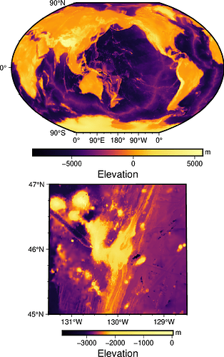
I am not sure why it is not working as expected (will look into it - it could be related to Allow for "makecpt" style colormap functionality in grdimage and colobar · Issue #372 · GenericMappingTools/pygmt · GitHub). In the meantime, you could write and read a colormap file as a workaround:

import pygmt

subset_region=[-131.5, -128.5, 45, 47] 
earth_relief_globe = pygmt.datasets.load_earth_relief(resolution="01d")
earth_relief_subset = pygmt.datasets.load_earth_relief("15s", region=subset_region)
fig = pygmt.Figure()
with fig.subplot(nrows=2, ncols=1, figsize=("15c", "15c"), margins="1c"):
    # Panel 1
    pygmt.grd2cpt(cmap="inferno", grid=earth_relief_globe, continuous=True, output="inferno_test_globe.cpt")
    fig.grdimage(grid=earth_relief_globe, projection="R", region="g", frame=True, panel=[0,0], cmap="inferno_test_globe.cpt")
    fig.colorbar(cmap="inferno_test_globe.cpt",frame=["a", "x+lElevation", "y+lm"])
    # Panel 2
    pygmt.grd2cpt(cmap="inferno",grid=earth_relief_subset, continuous=True, output="inferno_test_subset.cpt")
    fig.grdimage(grid=earth_relief_subset, projection="R", region=subset_region, frame=True, panel=[1,0], cmap="inferno_test_subset.cpt")
    fig.colorbar(cmap="inferno_test_subset.cpt", frame=["a", "x+lElevation", "y+lm"])
fig.show()

[andrebelem]

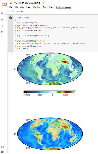
Strange… I just used the code of @seisman as pointed by @maxrjones above and it worked.
In this case GMT6 installed fresh with pygmt in colab notebook.

[maxrjones]

Yes, I think the difference is that it works as expected when using fig.shift_origin() but not when using fig.subplot().

[seisman]

Yes, I think the difference is that it works as expected when using fig.shift_origin() but not when using fig.subplot() .

I believe that’s one of the most non-intuitive parts for PyGMT!

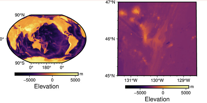
The example below is modified from @maxrjones’s example, without writing the CPT to a file. As mentioned by @maxrjones, it doesn’t work as expected. The two colorbars are the same.

### WRONG!!!! 
import pygmt

subset_region=[-131.5, -128.5, 45, 47] 
earth_relief_globe = pygmt.datasets.load_earth_relief(resolution="01d")
earth_relief_subset = pygmt.datasets.load_earth_relief("15s", region=subset_region)
fig = pygmt.Figure()
with fig.subplot(nrows=1, ncols=2, figsize=("15c", "15c"), margins="1c"):
    pygmt.grd2cpt(cmap="inferno", grid=earth_relief_globe, continuous=True)
    fig.grdimage(grid=earth_relief_globe, projection="R", region="g", frame=True, panel=0)
    fig.colorbar(frame=["a", "x+lElevation", "y+lm"])
    
    pygmt.grd2cpt(cmap="inferno",grid=earth_relief_subset, continuous=True)
    fig.grdimage(grid=earth_relief_subset, projection="R", region=subset_region, frame=True, panel=1)
    fig.colorbar(frame=["a", "x+lElevation", "y+lm"])
fig.show()

Here is the output:

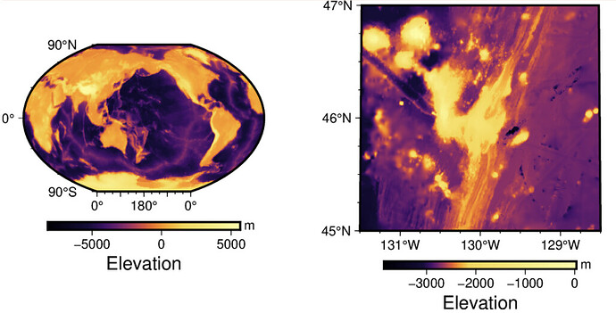
To plot the correct figure using fig.subplot(), you need to “activate” the panel (using fig.set_panel()) before creating the CPT. Here is the modified script:

### CORRECT!!!
import pygmt

subset_region=[-131.5, -128.5, 45, 47] 
earth_relief_globe = pygmt.datasets.load_earth_relief(resolution="01d")
earth_relief_subset = pygmt.datasets.load_earth_relief("15s", region=subset_region)
fig = pygmt.Figure()
with fig.subplot(nrows=1, ncols=2, figsize=("15c", "15c"), margins="1c"):
    with fig.set_panel(panel=0):
        pygmt.grd2cpt(cmap="inferno", grid=earth_relief_globe, continuous=True)
        fig.grdimage(grid=earth_relief_globe, projection="R", region="g", frame=True)
        fig.colorbar(frame=["a", "x+lElevation", "y+lm"])
    with fig.set_panel(panel=1):  
        pygmt.grd2cpt(cmap="inferno",grid=earth_relief_subset, continuous=True)
        fig.grdimage(grid=earth_relief_subset, projection="R", region=subset_region, frame=True)
        fig.colorbar(frame=["a", "x+lElevation", "y+lm"])
fig.show()

Here is the output：

To understand why these two are different, you need to know more about GMT’s Hierarchical Levels. In short, “a subplot” and a “panel” can have their own “current” CPT file. When there is no panel-level CPT file, the subplot-level CPT file will be used.

In the “wrong” example:

• the first grd2cpt function creates the “current” CPT for the current subplot, and it’s used by the first grdimage function in the first panel
• the 2nd grd2cpt creates a CPT file for the first panel (not the 2nd panel, because the 1st panel is currently activated!) Also, note that this CPT file is never used, as explained below.
• the 2nd grdimage is called in the 2nd panel. Because there is no panel-level CPT file for the 2nd panel, so the subplot-level CPT is used.

Thus both panels use the “subplot-level” CPT (created by the first grd2cpt call) and the colorbars are the same.

In the correct example, we first activate the panel using fig.set_panel() function, so grd2cpt creates panel-level CPT files for each panel. That’s why it works.

[TheGermanSquirrel]

Amazing, this solved it! Thanks!