Draping a Landsat8 RGB composite over SRTM

Dear all,

I am new in (Py)GMT. I am trying to drape a Landsat8 RGB composite over the SRTM DEM.
My Landsat8 composite RGB image is a GeoTIFF file. To start simple, however, I am trying with a single band.

In a Jupyter notebook, I do:

geographic_coordinates = {
'west': -4.17272200,
'north': 40.80833333,
'east': -3.03544243,
'south': 40.00833333,
}
gmt_coordinates=[
    geographic_coordinates['west'],
    geographic_coordinates['east'],
    geographic_coordinates['south'],
    geographic_coordinates['north'],
]
region = {
    'geographic': geographic_coordinates,
    'gmt': gmt_coordinates,
}

Get the relief

grid = pygmt.datasets.load_earth_relief(
    resolution="01m",
    region=region['gmt'],
    use_srtm=True,
)

and confirming it is what expected

fig = pygmt.Figure()
fig.grdview(
    grid=grid,
    # Set the azimuth to -130 (230) degrees and the elevation to 30 degrees
    perspective=[180, 90],
    frame=["xaf", "yaf", "WSnE"],
    projection="M15c",
    zsize="1.5c",
    surftype="s",
    cmap="geo",
    plane="1000+ggrey",
    # Set the contour pen thickness to "0.1p"
    contourpen="0.2p",
)
fig.show()

So far so good. How can I use a GeoTIFF file (say a single band to start with) with
fig.grdimage()? The following image is referenced in geographic coordinates (epsg:4326). Something like the following will crash the running (Jupyter) kernel, everytime.

fig.grdimage(grid=grid, img_in='madrid_landsat8_reflectance_5_2019_07_02T10_55_29_wgs84.tif')

I read the documentation and similar examples. For example https://docs.generic-mapping-tools.org/6.2/gallery/ex32.html where the image in question is converted to an nc format or this Q&A how-to-plot-satellite-optical-image-of-geotif-format-and-show-the-true-color and similar ones. I understand that I have to read-in or convert somehow the GeoTIFF image in some other format, like .ps (=Postscript?) or .nc.

I’d appreciate some help. Kindest regards, Nikos
Hi @NikosAlexandris, welcome to the forum!

So grdimage does support plotting single-band GeoTiff images directly (sorry if it’s not clear from the documentation). The img_in parameter is meant for something else (specifying the type of input grid). You could try to pass in your GeoTiff into the grid parameter directly using:

fig.grdimage(grid="madrid_landsat8_reflectance_5_2019_07_02T10_55_29_wgs84.tif")

If the above code doesn’t work, try posting the output of pygmt.grdinfo("madrid_landsat8_reflectance_5_2019_07_02T10_55_29_wgs84.tif") so we know what the data looks like.

As for plotting RGB composite maps, we’re hoping to get the grdmix function ready by PyGMT v0.5.0 (maybe October 2021?), you can see the related issue at Wrapper for grdmix · Issue #578 · GenericMappingTools/pygmt · GitHub and provide any feedback.

In the meantime, for plotting multi-band images, you can either call grdmix from the command-line using pure GMT, or using !grdmix if you’re in a jupyter notebook. The output of grdmix can then be passed directly to grdimage as usual.

1 Like

Thank you. Indeed, I can see now the/an image via

fig.grdimage(
    grid="../figures/madrid_landsat8_reflectance_r5_g3_b2_2019_07_02T10_55_29_wgs84.tif",
    frame='ag',
)
fig.show()

However, my goal is draping it over an SRTM. So, the following doesn’t work – in fact it seems to simply take forever:

fig = pygmt.Figure()
fig.grdview(
    grid=grid_1m,
    # Set the azimuth to -130 (230) degrees and the elevation to 30 degrees
    perspective=[180, 90],
    frame=["xaf", "yaf", "WSnE"],
    projection="M15c",
    zsize="1.5c",
    #surftype="i",
    cmap="geo",
    #plane="1000+ggrey",
    # Set the contour pen thickness to "0.1p"
    #contourpen="0.2p",
    drapegrid="../figures/madrid_landsat8_reflectance_r5_g3_b2_2019_07_02T10_55_29_wgs84.tif",
)
fig.show()

Any ideas?

Maybe try gdal to cut the image first.

The image’s extent is identically to the region coordinates I use (they are the ones set in GRASS GIS’ computational region, from which the images is exported – sidenote: almost any raster operation in GRASS GIS follows the currently set computational region).

Currently, this is not possible because GMT’s grdview operates on either a grid or three bands for R, G, and B but not composite images. For context and information about future plans, see https://github.com/GenericMappingTools/gmt/issues/5631.

For now, you would need to deconstruct the image into the R, G, and B bands and provide these to grdview. Here is an example that has worked for me, where !gmt grdmix ... executes an external gmt command to deconstruct the image (using Jupyter Notebook).

fig = pygmt.Figure()
region=[-106.5, -105.5, 39.7, 40]
!gmt grdmix truecolor.tif -D -Glayer_%c.nc
fig.grdview(grid="@earth_relief_01s",
            drapegrid="layer_R.nc -Glayer_G.nc -Glayer_B.nc",
            region=region,
            projection="M6i",
            frame=True,
            zsize="4c",
            perspective=[120, 40],
            surftype="i",
            verbose=True)
fig.show()

edit: One note about the argument passing multiple grids to drapegrid. This represents a short-term workaround. We’ve had some active discussions in both the GMT and PyGMT communities about the best way to support passing images to these plotting modules and hope to have a more intuitive solution for users soon.

1 Like

grdview -G accepts images, either indexed or RGB, but they need to cover exactly the same region as the grid (though can have different resolution). The RGB version, however, needs to be pixel interleaved I think.
Since Landsat comes in UTM and SRTM in geogs you’ll need to project one to fit the other.

Thanks. I am a bit puzzled with the .nc. Is this a GMT-specific format? GeoTIFFs not allowed here?
I missed the conversion line. But (why) is it necessary to convert to a netCDF format?
I have all source files, so I can do as I please – no need to decompose. In fact, I did convert the bands I want to netCDF. The blocker is now that it can’t find the nir.nc file for example. Hmmm?

Trying with one file first

region_gmt=region['gmt']
fig = pygmt.Figure()
fig.grdview(grid=grid_1m,
            drapegrid="nir.nc",
            region=region_gmt,
            projection="M6i",
            frame=True,
            perspective=[120, 40],
            surftype="i",
            verbose=True)
fig.show()

returns

GMTCLibError: Module 'grdview' failed with status code 72:
grdview [ERROR]: Cannot find file nir.nc

though the file is in the same directory as… Ah! ok, it works with the correct path. So does the following

region_gmt=region['gmt']
fig = pygmt.Figure()
fig.grdview(grid=grid_1m,
            drapegrid="../figures/nir.nc -G../figures/green.nc -G../figures/blue.nc",
            region=region_gmt,
            projection="M6i",
            frame=True,
            perspective=[120, 40],
            surftype="i",
            verbose=True)
fig.show()

Last remaining “task”: a proper colortable(s). Individual bands look just black and the composition of all appears brownish. So, it’s about getting it right for each individual band.

Already taken care. Thanks.

ps- By the way, in GRASS GIS’ terminology and database, a Location is defined by one and only one coordinate reference system (CRS). One can re-project data from<-> to other Locations, that is to other CRSes. So, my data are indeed in WGS84.

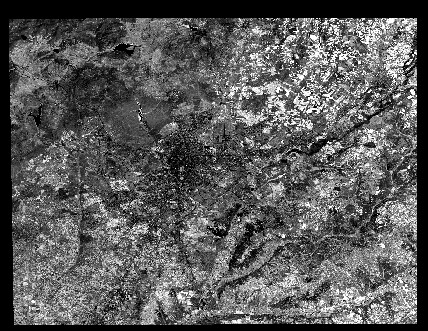
The original images (GeoTIFF files) look like the NIR band for example: NIR band

With

region_gmt=region['gmt']
fig = pygmt.Figure()
fig.grdview(grid=grid_1m,
            drapegrid="../figures/nir.nc -G../figures/green.nc -G../figures/blue.nc",
            region=region_gmt,
            projection="M6i",
            frame=True,
            perspective=[180, 40],
            zsize="2c",
            surftype="i",
            verbose=True)
fig.show()

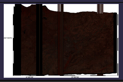
OK, here’s how it looks like: Landsat8 RGB over Madrid.
Issues to fix:

  • proper colors for each Landsat8 band
  • the zsize= gives some weird vertical columns/exaggerations.

You don’t. Any format that GDAL can ingest is good.

As an example I’ve improved the grdview Julia wrapper such that it can deal with images in any projection and extents (under the condition ofc that grid and image BoundingBox intercept).

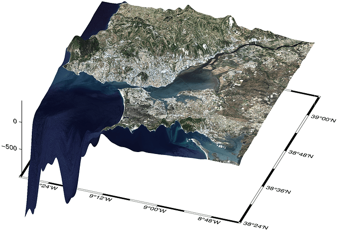
I’ve not a Madrid Landsat scene but I do have one over Lisboa for which the true color image was computed as explained in here or here. And the draping is as simple as

grdview("@earth_relief_01m", region=(-9.5,-8.7,38.4,39.1,-1000,400), drape="cor_verdadeira.tiff", zsize=4, view=(160,35), show=true)

note that the GeoTIFF image is in UTM and covers a much wider area than the one shown here.

I just failed to do the same (drape a satellite image over a grid) in other area. Could you share your image so I can check if there is a bug?

Here it is (155 MB)

You can also give a shot with my one-liner and your image.

1 Like

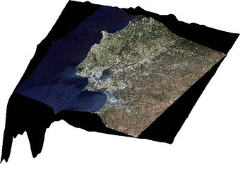
I get this figure with this one-line command:

gmt grdview @earth_relief_01m -R-9.5/-8.7/38.4/39.1/-1000/400 -JM14c -JZ4c -p160/35 -Qi -Gcor_verdadeira.tiff -Vi -png Lisboa

Is the same problem that we already know?

You can’t give an UTM image to drape on a geogs grid in plain GMT. You have to back project the UTM to geogs, cut it with the exact limits of the grid and then the plot will be correct.
The julia call does all that under the hood, and very efficiently.

1 Like

Thanks. I found the bug that appears with a -Gdrapeimage and -N+gcolor.