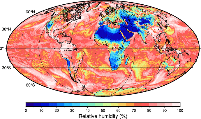
After a recent question on the use of gmt math I decided to investigate the grdmath module which is analogous to math, but for operating on grids instead. And what I found was very pleasing, so here is a simple example to demonstrate the sorts of things it can do.
The example presented is computing relative humidity of the air from grids of temperature and dew-point temperature. Some meteorological models only provide the temperature and dew-point temperature, so if one wants relative humidity, it is necessary to compute it from these two related variables.
The way to compute relative humidity is to use this formula:
where rh is the relative humidity in %, T_{d} is the dew-point temperature in ℃, T is the temperature in ℃ and e_{sat}(T) is the saturation vapour pressure of water at temperature T.
There are several equations for computing saturation vapour pressure. Tetens’ equation is a simple one which has an accuracy better than ±0.1% at temperatures normally encountered near the Earth’s surface (there are complications with sub-zero temperatures which we will not discuss here):
where e_{sat}(T) has units of hPa, and T has units of ℃.
Both math and grdmath support macros to simplify writing equations that use common formulae. So we start by defining some useful macros:
#!/usr/bin/env bash

# GMT grdmath macros.
cat << END > grdmath.macros
K2C = 273.15 SUB : Usage: tk K2C to return temperature in Celsius given temperature in Kelvin.
ESAT = STO@TC 17.27 MUL 237.3 RCL@TC ADD DIV EXP 6.1078 MUL : Usage tk ESAT to return saturation vapour pressure in hPa given temperature in Celsius using Tetens equation.
END
The first macro converts temperatures in Kelvin (the units usually used to disseminate temperature data) to Celsius. The second macro converts temperature in Celsius to saturation vapour pressure in hPa using Tetens’ equation.
I have gridded temperature and dew-point temperature data in NetCDF format from the European Centre for Medium-range Weather Forecasts. The grid extends from 180°W to 0° to 180°E, and from 90°S to 90°N, the spacing is 0,25° in both the longitude and latitude dimensions. The data are in a file called fld.nc, and the temperature and dew-point temperature variables are t2m and d2m respectively.
Here is the gmt grdmath command to compute the relative humidity (using the previously defined macros):
gmt grdmath fld.nc?d2m K2C ESAT fld.nc?t2m K2C ESAT DIV 100 MUL = rh_world.nc
And plotting it as well:
gmt begin rh_world PNG
	gmt grdmath fld.nc?d2m K2C ESAT fld.nc?t2m K2C ESAT DIV 100 MUL = rh_world.nc
	gmt makecpt -Chaxby -T0/100/5
	gmt grdimage rh_world.nc -JW15 -Rd -BWsen -Bpxf10a60g60 -Bpyf10a30g30
	gmt coast -Dl -Wthinnest,black
	gmt colorbar -Bpxf5a10+l"Relative humidity (%)" -DJCB+h+w12/0.3+jCT+o0/0.5
gmt end
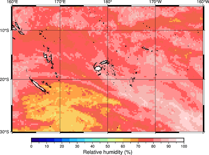
So far, so good. But here is the thing which really made me happy. The region I’m interested in crosses the International Dateline (180°E or thereabouts - it has some doglegs in it). Plotting data for an area which wraps from one edge of our grid to the other edge usually presents all sorts of hassles which need coding gymnastics to solve. But grdmath handles it seamlessly without any pain. Here is an example for the Southwest Pacific which crosses the edge of our grid:
gmt begin rh_swp PNG
	gmt grdmath -R160/200/-30/-5 fld.nc?d2m K2C ESAT fld.nc?t2m K2C ESAT DIV 100 MUL = rh_swp.nc
	gmt makecpt -Chaxby -T0/100/5
	gmt grdimage rh_swp.nc -JM15 -BWseN -Bpxf5a10g10 -Bpyf5a10g10
	gmt coast -Dh -Wthin,black
	gmt colorbar -Bpxf5a10+l"Relative humidity (%)" -DJCB+h+w12/0.3+jCT+o0/0.5
gmt end
There are more modern methods for doing this sort of computation - such as the Julia interface to GMT. But sometimes the old ways are pretty good too.

