GMT.jl: Quantile-weighted color bar & movie function

Cornec_H · May 14, 2024, 3:47pm

Hey everyone,
I am relatively new to Julia and very new to GMT and have run into a few problems that I have not been able to solve by reading the documentation.
I have a 19,000 x 153 matrix that I am reading in from a txt file. The first column is latitude, the second longitude and the rest of the columns are modeled average temperature in a given year.
I have managed to create the following map:

with this code:

data_points = [longitude latitude temp] # temp is temperature in year 1, i.e. data[:, 3]
grid = xyz2grd(data_points, region=(minimum(longitude), maximum(longitude), minimum(latitude), maximum(latitude)), spacing=(1.0, 1.0), method=:surface)
C = makecpt(cmap=:polar, range=(minimum(temp), maximum(temp)), continuous = true);
grdimage(grid, proj=:equidistCylindrical, frame=:af,cmap=C, title = "Temperature Distribution Map", colorbar = true)
coast!(region=:global, water="lightblue", proj=:equidistCylindrical, show = true).

Now to my questions:

The color scale is not very informative because it is currently uniform over the range. Is there a simple way in GMT.jl to take the quantile distribution into account instead? I have been experimenting with the auto=“ascl” argument inside grdimage but I receive the error message that “GMT: Expects a Matrix for input”.
Is there a way to automatically save this output to my desktop? I am currently saving the output from show = true manually. This would allow me to create a different png or jpg file for every year much faster.
How would I go about adapting what I have written to use the “movie” function in GMT.jl to create a video file that goes from year 1 to year 150? I tried to write a function that selected the correct temperature column based on the frame of “movie” but that does not seem to work.

Any help is greatly appreciated. I have listed my questions in order of importance. Please let me know if you need any additional information. This is also my first time asking. a question on a forum, so I am not entirely sure how much detail to give.

Thank you!

Joaquim · May 14, 2024, 6:17pm

Hi, welcome to the forum and let me say that for a first post it is very well made.

Since you dataset is global but data_points may not be (for example lacking points close to the poles because there missing points there), use regio=global. Also method=:surface does nothing because xyz2grd is not an interpolator but instead a reformater. It takes the x,y,z and reformat them in a grid. So:

grid = xyz2grd(data_points, region=:global, spacing=(1.0, 1.0))

I think the problem here is due to what seem to be data errors. Those < 40 degrees scattered points over Antarctica and those north of Greenland look very suspicious. Try:

C = makecpt(cmap=:polar, range=(-10, 30), continuous = true); # fine tune the limits.

and the there is also grd2cpt that computes a histogram equalized color map. e.g.

C = grd2cpt(grid)

Sorry, don’t know what is auto=“ascl”

Sure, use figname=blabla.jpg and that saves a jpg figure in current directory.

Should be possible but it has been long since a last looked into the GMT.jl movie function. Please post your trial code so I can look at it … later (don’t have much time in the next two days).

Esteban82 · May 14, 2024, 6:24pm

Is it me or your figure is greater than the frame? Look at the top of figure. It has no frame.

Joaquim · May 14, 2024, 6:45pm

I noticed that too and suspect that it’s due the xyz2grd computed grid not having an R=-180/180/-90/90 (because region was got from data’s min/max)

Cornec_H · May 15, 2024, 3:14pm

Thank you both so much! I have managed to save all the maps using the following function:


function MakeTempMaps()
    cd("~Plots/Average Temperature")
    latitude = datamatrix[:, 2]
    longitude = datamatrix[:, 3]
    df1 = [longitude latitude datamatrix[:,4]]
    grd1 = xyz2grd(df1, region=(-180, 180, -60, 75), spacing=(1.0, 1.0))
    C = grd2cpt(grd1, cmap=:polar);
    for i in 1:150
        temp = datamatrix[:,i+3]
        data_points = [longitude latitude temp]
        grid = xyz2grd(data_points, region=(-180, 180, -60, 75), spacing=(1.0, 1.0))

        grdimage(grid, proj=:equidistCylindrical, frame=:af,cmap=C, title = "Temperature Distribution Map ("*string(i+1989)*")", colorbar = true)
        coast!(region=(-180, 180, -60, 75), water="lightblue", proj=:equidistCylindrical, savefig = string(i+1989)*".jpg")
    end
    cd(fig_path)
end
MakeTempMaps()

The maps now look like this:

Thank you again for your help. If there is a simple way to use the movie function to create an mp4 out of the images, that would be great, but otherwise I can probably use some other package to string the jpg files together.

One last thing: Is there a cmap argument or color palette (both in color and black/white) with higher contrasts that is easier to read or that you recommend? I am not entirely satisfied with “cmap = polar”.

Thank you for all your suggestions!
Regards

Esteban82 · May 15, 2024, 3:23pm

Rigth now, the only option within GMT is to use bash scripts.

Joaquim · May 15, 2024, 3:39pm

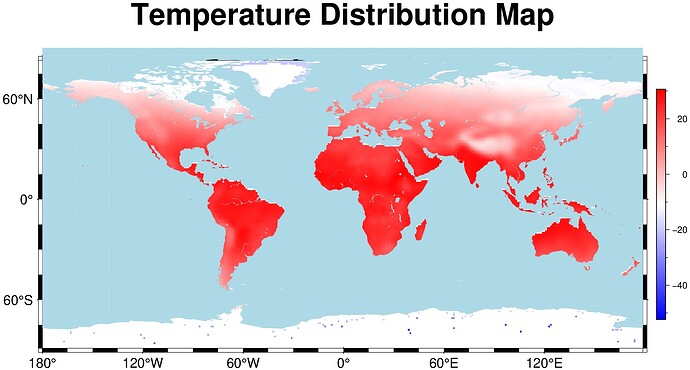
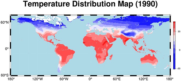
Funny that all of sudden two persons (the other one here) are asking about movies with GMT.jl

Yes, it possible to do (some) movies with GMT.jl but I have not looked at it in a long time so I would not be surprised if some things have broken (though, the simple CI test are still passing).

I don’t know what the variable datamatrix contains but it is is a GMTdataset (one that we get when reading data with gmtread) code can be made more elegant by using the xvar="x column name" and same for yvar).

There are tons of color maps (CPTs) in GMT. This is a quick list (lazzy, and time shortage to look in the GMT “Technical reference” page). This is what we get by running makecpt on the command line

     gmt/abyss          : Black/dark blue to lightblue for bathymetry [R=-8000/0, C=RGB]
     gmt/bathy          : Like abyss but via aquamarine at mid-depths [R=-8000/0, C=RGB]
     gmt/categorical    : Color table particularly suitable for categorical data [C=RGB]
     gmt/cyclic         : Cyclic colormap, spans 360 degrees of hue [C=HSV]
     gmt/dem2           : Digital Elevation Model (DEM) scale by Dewez/Wessel [R=0/4900, C=RGB]
     gmt/dem3           : Digital Elevation Model (DEM) scale by Paul Wessel [R=0/6000, C=RGB]
     gmt/drywet         : Goes from dry to wet colors [C=RGB]
     gmt/earth          : Colors for global bathymetry/topography relief [R=-11000/9000, H, C=RGB]
     gmt/etopo1         : Colormap used in the ETOPO1 global relief map [R=-11000/8500, H, C=RGB]
     gmt/gebco          : Colors for GEBCO bathymetric charts [R=-7000/0, C=RGB]
     gmt/geo            : Colors for global bathymetry/topography relief [R=-8000/8000, H, C=RGB]
     gmt/globe          : Colors for global bathymetry/topography relief [R=-10000/10000, H, C=RGB]
     gmt/gray           : Gray linear ramp from black to white [C=RGB]
     gmt/haxby          : Bill Haxby's color scheme for geoid & gravity [C=RGB]
     gmt/ibcso          : The IBCSO bathymetry colors [R=-12000/0, C=RGB]
     gmt/mag            : Colors for magnetic anomaly maps [R=-2000/2000, H, C=RGB]
     gmt/nighttime      : Colors for DMSP-OLS Nighttime Lights Time Series [C=HSV]
     gmt/no_green       : For those who hate green [S, C=RGB]
     gmt/ocean          : White-green-blue bathymetry scale [R=-8000/0, C=RGB]
     gmt/paired         : Categorical color map with 6 pairs of colors [C=RGB]
     gmt/rainbow        : Rainbow, magenta-blue-cyan-green-yellow-red [C=HSV]
     gmt/red2green      : Polar scale from red to green via white [S, C=RGB]
     gmt/relief         : Wessel/Martinez colors for topography [R=-8000/+8000, H, C=RGB]
     gmt/rust2silver    : USGS color map for planets such as Mercury [R=-5500/5500, C=RGB]
     gmt/seafloor       : Purple-blue-white bathymetry scale [R=-6000/0, C=RGB]
     gmt/sealand        : Smith bathymetry/topography scale [R=-6000/+3000, H, C=HSV]
     gmt/seis           : R-O-Y-G-B seismic tomography colors [C=RGB]
     gmt/split          : Like polar, but via black instead of white [S, C=RGB]
     gmt/srtm           : Like dem2, but with blue for oceans [H, C=RGB]
     gmt/terra          : Colors for global bathymetry/topography relief [R=-7000/7000, H, C=RGB]
     gmt/topo           : Sandwell/Anderson colors for topography [R=-7000/+7000, H, C=HSV]
     gmt/world          : Colors for global bathymetry/topography relief [R=-7000/7000, H, C=RGB]
     gmt/wysiwyg        : 20 well-separated RGB colors [C=RGB]
     SCM/acton          : Perceptually uniform sequential colormap, by Fabio Crameri [C=RGB]
     SCM/actonS         : Perceptually uniform sequential categorical colormap, by Fabio Crameri [C=RGB]
     SCM/bam            : Perceptually uniform bimodal colormap, light, by Fabio Crameri [C=RGB]
     SCM/bamO           : Perceptually uniform bimodal cyclic colormap, light, by Fabio Crameri [C=RGB]
     SCM/bamako         : Perceptually uniform, low-lightness gradient colormap by Fabio Crameri [C=RGB]
     SCM/bamakoS        : Perceptually uniform, low-lightness gradient categorical colormap by Fabio Crameri [C=RGB]
     SCM/batlow         : Perceptually uniform sequential 'rainbow' colormap by, Fabio Crameri [C=RGB]
     SCM/batlowK        : Perceptually uniform 'rainbow' colormap with black ending by Fabio Crameri [C=RGB]
     SCM/batlowS        : Perceptually uniform 'rainbow' categorical colormap by Fabio Crameri [C=RGB]
     SCM/batlowW        : Perceptually uniform 'rainbow' colormap with white ending by Fabio Crameri [C=RGB]
     SCM/berlin         : Perceptually uniform bimodal colormap, dark, by Fabio Crameri [S, C=RGB]
     SCM/bilbao         : Perceptually uniform colormap by Fabio Crameri [C=RGB]
     SCM/bilbaoS        : Perceptually uniform categorical colormap by Fabio Crameri [C=RGB]
     SCM/broc           : Perceptually uniform bimodal colormap, light, by Fabio Crameri [S, C=RGB]
     SCM/brocO          : Perceptually uniform bimodal cyclic colormap, light, by Fabio Crameri [C=RGB]
     SCM/buda           : Perceptually uniform, low-lightness gradient colormap, by Fabio Crameri [C=RGB]
     SCM/budaS          : Perceptually uniform, low-lightness gradient categorical colormap, by Fabio Crameri [C=RGB]
     SCM/bukavu         : Perceptually uniform multi-sequential colormap by Fabio Crameri [H,C=RGB]
     SCM/cork           : Perceptually uniform bimodal colormap, light, by Fabio Crameri [S, C=RGB]
     SCM/corkO          : Perceptually uniform bimodal cyclic colormap, light, by Fabio Crameri [C=RGB]
     SCM/davos          : Perceptually uniform colormap by Fabio Crameri [C=RGB]
     SCM/davosS         : Perceptually uniform categorical colormap by Fabio Crameri [C=RGB]
     SCM/devon          : Perceptually uniform sequential colormap, by Fabio Crameri [C=RGB]
     SCM/devonS         : Perceptually uniform sequential categorical colormap, by Fabio Crameri [C=RGB]
     SCM/fes            : Perceptually uniform multi-sequential colormap by Fabio Crameri [H,C=RGB]
     SCM/glasgow        : Perceptually uniform sequential colormap by Fabio Crameri [C=RGB]
     SCM/grayC          : Perceptually uniform 'gray' colormap, by Fabio Crameri [C=RGB]
     SCM/grayCS         : Perceptually uniform 'gray' categorical colormap by Fabio Crameri [C=RGB]
     SCM/hawaii         : Perceptually uniform sequential colormap, by Fabio Crameri [C=RGB]
     SCM/hawaiiS        : Perceptually uniform lush categorical colormap by Fabio Crameri [C=RGB]
     SCM/imola          : Perceptually uniform, low-lightness gradient colormap, by Fabio Crameri [C=RGB]
     SCM/imolaS         : Perceptually uniform, low-lightness gradient categorical colormap, by Fabio Crameri [C=RGB]
     SCM/lajolla        : Perceptually uniform colormap, without black or white, by Fabio Crameri [C=RGB]
     SCM/lajollaS       : Perceptually uniform categorical colormap, without black or white, by Fabio Crameri [C=RGB]
     SCM/lapaz          : Perceptually uniform 'rainbow' colormap, by Fabio Crameri [C=RGB]
     SCM/lapazS         : Perceptually uniform 'rainbow' categorical colormap by Fabio Crameri [C=RGB]
     SCM/lipari         : Perceptually uniform sequential colormap by Fabio Crameri [C=RGB]
     SCM/lisbon         : Perceptually uniform bimodal colormap, dark, by Fabio Crameri [S, C=RGB]
     SCM/managua        : Perceptually uniform diverging colormap, by Fabio Crameri [S,C=RGB]
     SCM/navia          : Perceptually uniform sequential colormap by Fabio Crameri [C=RGB]
     SCM/nuuk           : Perceptually uniform, low-lightness gradient colormap, by Fabio Crameri [C=RGB]
     SCM/nuukS          : Perceptually uniform, low-lightness gradient categorical colormap, by Fabio Crameri [C=RGB]
     SCM/oleron         : Perceptually uniform topography colormap, by Fabio Crameri [H, C=RGB]
     SCM/oslo           : Perceptually uniform, black & white limits, by Fabio Crameri [C=RGB]
     SCM/osloS          : Perceptually uniform, B&W limits, categorical colormap, by Fabio Crameri [C=RGB]
     SCM/roma           : Perceptually uniform 'seis' colormap, by Fabio Crameri [S, C=RGB]
     SCM/romaO          : Perceptually uniform cyclic colormap by Fabio Crameri [C=RGB]
     SCM/tofino         : Perceptually uniform bimodal colormap, dark, by Fabio Crameri [S, C=RGB]
     SCM/tokyo          : Perceptually uniform colormap without black or white, by Fabio Crameri [C=RGB]
     SCM/tokyoS         : Perceptually uniform categorical colormap without black or white, by Fabio Crameri [C=RGB]
     SCM/turku          : Perceptually uniform colormap by Fabio Crameri [C=RGB]
     SCM/turkuS         : Perceptually uniform categorical colormap by Fabio Crameri [C=RGB]
     SCM/vanimo         : Perceptually uniform bimodal colormap, dark, by Fabio Crameri [C=RGB]
     SCM/vik            : Perceptually uniform bimodal colormap, light, by Fabio Crameri [S, C=RGB]
     SCM/vikO           : Perceptually uniform bimodal cyclic colormap, light, by Fabio Crameri [C=RGB]
     cmocean/algae      : Perceptually uniform colormap, by Kirsten Thyng [C=RGB]
     cmocean/amp        : Perceptually uniform colormap, by Kirsten Thyng [C=RGB]
     cmocean/balance    : Perceptually uniform divergent colormap, by Kirsten Thyng [S,C=RGB]
     cmocean/curl       : Perceptually uniform divergent colormap, by Kirsten Thyng [S,C=RGB]
     cmocean/deep       : Perceptually uniform colormap, by Kirsten Thyng [C=RGB]
     cmocean/delta      : Perceptually uniform divergent colormap, by Kirsten Thyng [S,C=RGB]
     cmocean/dense      : Perceptually uniform colormap, by Kirsten Thyng [C=RGB]
     cmocean/diff       : Perceptually uniform divergent colormap, by Kirsten Thyng [S,C=RGB]
     cmocean/gray       : Perceptually uniform grayscale map, by Kirsten Thyng [C=RGB]
     cmocean/haline     : Perceptually uniform colormap, by Kirsten Thyng [C=RGB]
     cmocean/ice        : Perceptually uniform colormap, by Kirsten Thyng [C=RGB]
     cmocean/matter     : Perceptually uniform colormap, by Kirsten Thyng [C=RGB]
     cmocean/oxy        : Perceptually uniform divergent colormap, by Kirsten Thyng [C=RGB]
     cmocean/phase      : Perceptually uniform cyclic colormap, by Kirsten Thyng [O,C=RGB]
     cmocean/rain       : Perceptually uniform colormap, by Kirsten Thyng [C=RGB]
     cmocean/solar      : Perceptually uniform colormap, by Kirsten Thyng [C=RGB]
     cmocean/speed      : Perceptually uniform colormap, by Kirsten Thyng [C=RGB]
     cmocean/tarn       : Perceptually uniform colormap, by Kirsten Thyng [S,C=RGB]
     cmocean/tempo      : Perceptually uniform colormap, by Kirsten Thyng [C=RGB]
     cmocean/thermal    : Perceptually uniform colormap, by Kirsten Thyng [C=RGB]
     cmocean/topo       : Perceptually uniform colormap, by Kirsten Thyng [H,C=RGB]
     cmocean/turbid     : Perceptually uniform colormap, by Kirsten Thyng [C=RGB]
     cpt-city/cubhelix  : Intensity colormap via cube helix by Dave Green [C=RGB]
     cpt-city/dem1      : Digital Elevation Model (DEM) scale by Thomas Dewez [R=0/800, C=RGB]
     cpt-city/dem4      : Digital Elevation Model (DEM) scale for Wikipedia figures [R=0/1500, C=RGB]
     cpt-city/elevation : Washed-out colors for topography [R=0/7000, C=RGB]
     google/turbo       : Google's Improved Rainbow Colormap for Visualization [C=RGB]
     matlab/cool        : Linear change from blue to magenta [C=RGB]
     matlab/copper      : Dark to light copper brown [C=RGB]
     matlab/hot         : Black through red and yellow to white [C=RGB]
     matlab/jet         : Dark to light blue, white, yellow and red [C=RGB]
     matlab/polar       : Blue via white to red [S, C=RGB]
     matplotlib/inferno : New colormap Option B from matplotlib [C=RGB]
     matplotlib/magma   : New colormap Option A from matplotlib [C=RGB]
     matplotlib/plasma  : New colormap Option C from matplotlib [C=RGB]
     matplotlib/viridis : New colormap Option D from matplotlib [C=RGB]
     panoply/panoply    : Default colormap from the Panoply application [C=RGB]

jjg · May 15, 2024, 3:49pm

Lots of cpt-files at cpt-city.

Cornec_H · May 15, 2024, 5:10pm

Thank you all!

In case somebody looks for a solution in the future, I will add a bit of code here that creates an mp4 file from a group of png files without using movies.


using VideoIO, FileIO, ImageTransformations


# Set the path to the directory containing the png images
dir = ""  

imgnames = filter(x->occursin(".png",x), readdir(dir)) # Populate list of all .pngs
intstrings =  map(x->split(x,".")[1], imgnames) # Extract index from filenames
p = sortperm(parse.(Int, intstrings)) #sort files numerically
imgnames = imgnames[p]

encoder_options = (crf=23, preset="medium")
firstimg = load(joinpath(dir, imgnames[1]))
img_resized = imresize(firstimg,(512, 768)); # Needed to resize images because GMT.grdimage saves them in 845 x 1861 resolution.
open_video_out("video.mp4", img_resized, framerate=5, encoder_options=encoder_options) do writer
    @showprogress "Encoding video frames.." for i in eachindex(imgnames)
        img = load(joinpath(dir, imgnames[i]))
        img_res = imresize(img,(512, 768));
        write(writer, img_res)
    end
end

Thank you for the cpt list and have a great rest of your day.

Joaquim · May 16, 2024, 12:53pm

Would this movie recipe avoid that step?

Joaquim · May 17, 2024, 2:25pm

See also this post. It should cover your case too.