Grdimage not plotting entire dataset:

Hi All -

I have been plotting .grd files and for some reason the highest latitude position in my file are either not being read or are just not plotting. I know that the data in the file are valid and are within the cpt I made for these plots. Here is a small sample of the .grd file.

-114.40000 62.20000 4.028
-114.20000 62.20000 4.028
-114.00000 62.20000 4.028
-113.80000 62.20000 4.028
-113.60000 62.20000 4.028
-113.40000 62.20000 4.028
-113.20000 62.20000 4.028
-113.00000 62.20000 4.028
-112.80000 62.20000 3.842
-114.40000 62.40000 4.028
-114.20000 62.40000 4.028
-114.00000 62.40000 3.842

This lon/lat is up around Yellowknife in central Canada.

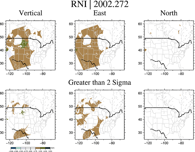
As an example, here is one of the plots. You can see that there is a line that cuts below where that the above lon/lat is specified โ€“ and that is true for every plot I make even though there is data that should be plotted around the Yellowknife area. I canโ€™t seem to figure out why this is happening.

To the best of my knowledge, Iโ€™m not clipping any regions, and Iโ€™ve specified that my region is 2-degrees higher at 64-degree latitude to ensure that my plot would include the entirety of my data.

Here is the section of the .grd file for the plot shown above, which should, again, be shown in the plot, but is absent:

-114.40000 62.20000 1.088
-114.20000 62.20000 1.088
-114.00000 62.20000 1.088
-113.80000 62.20000 1.088
-113.60000 62.20000 1.088
-113.40000 62.20000 1.088
-113.20000 62.20000 1.088
-113.00000 62.20000 1.088
-112.80000 62.20000 0
-114.40000 62.40000 1.088
-114.20000 62.40000 1.088
-114.00000 62.40000 1.088

And here is the code I have written to create the above plot:

    GMT.subplot(grid = "2x3", 
        title = "RNI | $yr",
        clearance = (top = 0.5), 
        savefig = imgpath * "$count_up" * ".png"); 
        
        # rad
        GMT.grdimage(sigrad, (region= [-130 -70 24 64], proj=:Winkel),
        coast = (borders = ((type = 1, pen = ("thick", "black")), (type = 2, pen = ("thinner", "lightgrey"))),
            area = 500,
            shore = (:thinnest, :lightgrey)),
        cmap = bukavu,
        panel = (1,1),
        title = "Vertical"
        );


        GMT.grdimage(sigsigrad, (region= [-130 -70 24 64], proj=:Winkel),
        coast = (borders = ((type = 1, pen = ("thick", "black")), (type = 2, pen = ("thinner", "lightgrey"))),
            area = 500,
            shore = (:thinnest, :lightgrey)),
        cmap = bukavu,
        panel = (2,1)
        );

        # lon
        GMT.grdimage(siglon, (region= [-130 -70 24 64], proj=:Winkel),
        coast = (borders = ((type = 1, pen = ("thick", "black")), (type = 2, pen = ("thinner", "lightgrey"))),
            area = 500,
            shore = (:thinnest, :lightgrey)),
        cmap = bukavu,
        panel = (1,2),
        title = "East"
        );

        GMT.grdimage(sigsiglon, (region= [-130 -70 24 64], proj=:Winkel),
        coast = (borders = ((type = 1, pen = ("thick", "black")), (type = 2, pen = ("thinner", "lightgrey"))),
            area = 500,
            shore = (:thinnest, :lightgrey)),
        cmap = bukavu,
        panel = (2,2),
        title = "Greater than 2 Sigma"
        );

        # lat
        GMT.grdimage(siglat, (region= [-130 -70 24 64], proj=:Winkel),
        coast = (borders = ((type = 1, pen = ("thick", "black")), (type = 2, pen = ("thinner", "lightgrey"))),
            area = 500,
            shore = (:thinnest, :lightgrey)),
        cmap = bukavu,
        panel = (1,3),
        title = "North"
        );

        GMT.grdimage(sigsiglat, (region= [-130 -70 24 64], proj=:Winkel),
        coast = (borders = ((type = 1, pen = ("thick", "black")), (type = 2, pen = ("thinner", "lightgrey"))),
            area = 500,
            shore = (:thinnest, :lightgrey)),
        cmap = bukavu,
        panel = (2,3)
        );

        colorbar!(position=(outside=true, anchor=:BC), equal=true, cmap=bukavu, ylabel = "mm");

Here is a link for the data via proton drive, if you would like to check out the complete data for this epoch.

If that link doesnโ€™t work for any reason, feel free to PM me and I can send you the data via email if youโ€™re so inclined.

Thank you for any help or insight :slight_smile:

  • Rob

EDIT: The fact that the columns I copy & pasted are showing up red in this seems weird. Could the reason behind the columns being shown in red here be a clue to as to why my data is not plotting? Iโ€™m not sure why those would be a problem though. The rest of the columns are formatted the same way, and the lon/lat are within my map region too. :person_shrugging:

Sorry but I miss to see whatโ€™s missing. Please reduce you questions to a minimum example. A single plot (ideally with a one-liner when possible) should be enough to demonstrate a problem.

This all look good to me.

julia> grdinfo("2002.272_rad.grd")
10-element Vector{String}:
 "2002.272_rad.grd: Title: Grid imported via GDAL"
 "2002.272_rad.grd: Command: "
 "2002.272_rad.grd: Remark: "
 "2002.272_rad.grd: Gridline node registration used [Cartesian grid]"
 "2002.272_rad.grd: Grid file format: gd = Import/export through GDAL"
 "2002.272_rad.grd: x_min: -124.6 x_max: -64.8 x_inc: 0.2 name: x n_columns: 300"
 "2002.272_rad.grd: y_min: 24.8 y_max: 62.4 y_inc: 0.2 name: y n_rows: 189"
 "2002.272_rad.grd: v_min: -2.056 v_max: 4.927 name: z"
 "2002.272_rad.grd: scale_factor: 1 add_offset: 0"
 "2002.272_rad.grd: Default CPT: "

julia> gmtinfo("2002.272_rad.grd")
1-element Vector{String}:
 "2002.272_rad.grd: N = 42440\t<-124.6/-64.8>\t<24.8/62.4>\t<-2.056/4.927>"

and this too

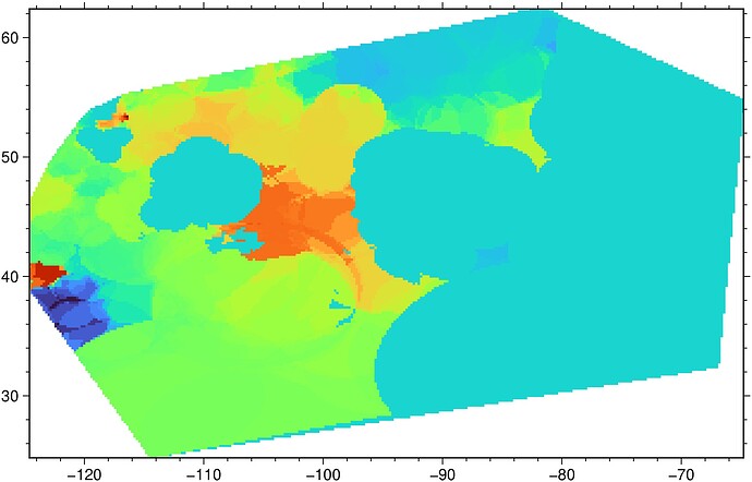
viz("2002.272_rad.grd")

The lon/lat of -116, 62 on your plot is missing too. There should be data plotted up around the -116, 62 region.

Unless Iโ€™m not understanding something?

If you scroll down to the bottom of the file I provided, youโ€™ll see that there is a value at -114.00, 62.4, which is not shown in your plot either.

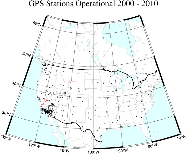
Perhaps It will be easier to see if I provide another reference photo of the GPS stations that are being interpolated.

The highest latitude station in the above plot has data, and is not being plotted in my, or in your plot. Thatโ€™s what Iโ€™m trying to figure out.

Because there is nothing on that gridโ€™s cell

julia> grdtrack("2002.272_rad.grd", [-116 62], n=:n)

1ร—3 GMTdataset{Float64, 2}
 Row โ”‚      X     Y    Z
โ”€โ”€โ”€โ”€โ”€โ”ผโ”€โ”€โ”€โ”€โ”€โ”€โ”€โ”€โ”€โ”€โ”€โ”€โ”€โ”€โ”€โ”€โ”€โ”€โ”€
   1 โ”‚ -116.0  62.0  NaN

Iโ€™m so confused. How do you have an NaN? I downloaded the file I uploaded to double check, and it contains no NaN entries.

The very last rows, which are the highest latitudes, I have these values:

-114.60000 62.20000 1.088
-114.40000 62.20000 1.088
-114.20000 62.20000 1.088
-114.00000 62.20000 1.088
-113.80000 62.20000 1.088
-113.60000 62.20000 1.088
-113.40000 62.20000 1.088
-113.20000 62.20000 1.088
-113.00000 62.20000 1.088
-112.80000 62.20000 0
-114.40000 62.40000 1.088
-114.20000 62.40000 1.088
-114.00000 62.40000 1.088

Which are missing from both yours and my plots.

I think my file is being read incorrectly โ€“ or itโ€™s formatted incorrectly?

julia> epoch = gmtread("/home/rob/Desktop/2002.272_rad.grd")
A GMTgrid object with 1 layers of type Float32
title: Grid imported via GDAL
Gridline node registration used
x_min: -124.6	x_max :-64.79999999999998	x_inc :0.20000000000000004	n_columns :300
y_min: 24.8	y_max :62.4	y_inc :0.19999999999999998	n_rows :189
z_min: -2.055999994277954	z_max :4.927000045776367
Mem layout:	BCB

julia> epoch[:,1]
189-element Vector{Float32}:
 NaN
 NaN
 NaN
 NaN
 NaN
 NaN
 NaN
 NaN
 NaN
 NaN
 NaN
 NaN
   โ‹ฎ
 NaN
 NaN
 NaN
 NaN
 NaN
 NaN
 NaN
 NaN
 NaN
 NaN
 NaN
 NaN

The file 2002.272_rad.grd, which is a grid in text with no metadata whatsoever and hence relies in GDAL figure it out, has 42440 rows (points) but the inferred grid (see above) has dims 300 x 189 = 56700 nodes. The difference are missing data, represented internally by NaNs.

See

julia> grd2xyz("2002.272_rad.grd")
BoundingBox: [-124.6, -64.79999999999998, 24.8, 62.4, -2.055999994277954, 4.927000045776367]

56700ร—3 GMTdataset{Float64, 2}
   Row โ”‚  col.1  col.2  col.3
โ”€โ”€โ”€โ”€โ”€โ”€โ”€โ”ผโ”€โ”€โ”€โ”€โ”€โ”€โ”€โ”€โ”€โ”€โ”€โ”€โ”€โ”€โ”€โ”€โ”€โ”€โ”€โ”€โ”€โ”€
     1 โ”‚ -124.6   62.4    NaN
     2 โ”‚ -124.4   62.4    NaN
     3 โ”‚ -124.2   62.4    NaN
     4 โ”‚ -124.0   62.4    NaN
     5 โ”‚ -123.8   62.4    NaN
     6 โ”‚ -123.6   62.4    NaN
     7 โ”‚ -123.4   62.4    NaN
     8 โ”‚ -123.2   62.4    NaN
     9 โ”‚ -123.0   62.4    NaN
    10 โ”‚ -122.8   62.4    NaN
    11 โ”‚ -122.6   62.4    NaN
    12 โ”‚ -122.4   62.4    NaN
   โ‹ฎ   โ”‚   โ‹ฎ       โ‹ฎ      โ‹ฎ
 56690 โ”‚  -66.8   24.8    NaN
 56691 โ”‚  -66.6   24.8    NaN
 56692 โ”‚  -66.4   24.8    NaN
 56693 โ”‚  -66.2   24.8    NaN
 56694 โ”‚  -66.0   24.8    NaN
 56695 โ”‚  -65.8   24.8    NaN
 56696 โ”‚  -65.6   24.8    NaN
 56697 โ”‚  -65.4   24.8    NaN
 56698 โ”‚  -65.2   24.8    NaN
 56699 โ”‚  -65.0   24.8    NaN
 56700 โ”‚  -64.8   24.8    NaN
            56677 rows omitted

now skip the NaNs

julia> grd2xyz("2002.272_rad.grd", s=true)
BoundingBox: [-124.6, -64.79999999999998, 24.8, 62.4, -2.055999994277954, 4.927000045776367]

42440ร—3 GMTdataset{Float64, 2}
   Row โ”‚  col.1  col.2   col.3
โ”€โ”€โ”€โ”€โ”€โ”€โ”€โ”ผโ”€โ”€โ”€โ”€โ”€โ”€โ”€โ”€โ”€โ”€โ”€โ”€โ”€โ”€โ”€โ”€โ”€โ”€โ”€โ”€โ”€โ”€โ”€
     1 โ”‚  -82.6   62.4  -0.07
     2 โ”‚  -82.4   62.4  -0.07
     3 โ”‚  -82.2   62.4  -0.07
     4 โ”‚  -82.0   62.4  -0.07
     5 โ”‚  -81.8   62.4  -0.07
     6 โ”‚  -81.6   62.4  -0.1
     7 โ”‚  -81.4   62.4  -0.1
     8 โ”‚  -81.2   62.4   0.0
     9 โ”‚  -83.6   62.2  -0.07
    10 โ”‚  -83.4   62.2  -0.07
    11 โ”‚  -83.2   62.2  -0.07
    12 โ”‚  -83.0   62.2  -0.07
   โ‹ฎ   โ”‚   โ‹ฎ       โ‹ฎ      โ‹ฎ
 42430 โ”‚ -114.2   25.0   1.088
 42431 โ”‚ -114.0   25.0   1.088
 42432 โ”‚ -113.8   25.0   1.088
 42433 โ”‚ -113.6   25.0   1.088
 42434 โ”‚ -113.4   25.0   1.088
 42435 โ”‚ -113.2   25.0   1.088
 42436 โ”‚ -113.0   25.0   1.088
 42437 โ”‚ -112.8   25.0   0.0
 42438 โ”‚ -114.4   24.8   1.088
 42439 โ”‚ -114.2   24.8   1.088
 42440 โ”‚ -114.0   24.8   1.088

Okay, that makes sense. The .grd doesnโ€™t have any metadata probably because I made the file myself with a bash script using awk commands.

But, even with the NaNs, which I understand where they are coming from now, still leaves me with the initial problem I was having of the data that is present at the coordinate of -114, 62.4 (and others around that region) is still not being shown on the map. Unless those points are being turned into NaN values for some reason in the process?

But itโ€™s true that if I do

julia> G = xyz2grd("2002.272_rad.grd", I=0.2, region="-124.6/-64.8/24.8/62.4")
A GMTgrid object with 1 layers of type Float32
command: gmt xyz2grd 2002.272_rad.grd -I0.2 -R-124.6/-64.8/24.8/62.4 -JX15c/10c -G@GMTAPI@-S-O-G-G-G-N-000085 -f0f,1f
Gridline node registration used
x_min: -124.6   x_max :-64.8    x_inc :0.19999999999999998      n_columns :300
y_min: 24.8     y_max :62.4     y_inc :0.19999999999999998      n_rows :189
z_min: -2.055999994277954       z_max :4.927000045776367

and

julia> grdtrack(G, [-114 62.4])
grdtrack [WARNING]: Some input points were outside the grid domain(s).
String[]

Here the grid was created by GMT, not GDAL (as in your case) and upper row (lat = 62.4) does not seem to be well represented, See how y_inc :0.19999999999999998 and not exactly = 0.2.

and

julia> grdtrack(G, [-114 62.39999999])

1ร—3 GMTdataset{Float64, 2}
 Row โ”‚      X     Y      Z
โ”€โ”€โ”€โ”€โ”€โ”ผโ”€โ”€โ”€โ”€โ”€โ”€โ”€โ”€โ”€โ”€โ”€โ”€โ”€โ”€โ”€โ”€โ”€โ”€โ”€โ”€โ”€
   1 โ”‚ -114.0  62.4  1.088

Not sure what is happening here.

hmm, okay, some kind of floating-point conversion error? maybe If I use Juliaโ€™s round() operation it will help alleviate it. Guess Iโ€™ll try it out.

Yes, Iโ€™m also thinking in some floating point issue that we fell into. When I save the grid on disk in netCDF and see in in netCDF viewer I see that the lat element y vector is not exactly equal to 62.4, which is normal due to the floating point representation but this seems also to interfere with the ability to get the last cell. All too weird.

My suggestion for now is to add an empty row at the top of the grid (with NaNs).

Gotcha. Iโ€™ll give that a go and see what I come up with. As always, thank you for all the help Joaquim!

Found a better solution. Save your grids in pixel registration. Something like this

G = xyz2grd("2002.272_rad.grd", I=0.2, region="-124.7/-64.7/24.7/62.5", r=:p);
G.proj4="";    # To workaround a kind of bug I just found in `xyz2grd`
gmtwrite("name.grd", G) 

and then use the name.grd instead. With it now I get

julia> grdtrack(G, [-114 62.4])

1ร—3 GMTdataset{Float64, 2}
 Row โ”‚      X     Y      Z
โ”€โ”€โ”€โ”€โ”€โ”ผโ”€โ”€โ”€โ”€โ”€โ”€โ”€โ”€โ”€โ”€โ”€โ”€โ”€โ”€โ”€โ”€โ”€โ”€โ”€โ”€โ”€
   1 โ”‚ -114.0  62.4  1.088
1 Like

Youโ€™re a wizard.

My implementation of round() did not work. I didnโ€™t really expect it to. lol

Iโ€™ll give your above recommendation a try right now.

The case may be more serious. The automatic conversion via GDAL seems to be upside-down.

See this plot that overlap the points themselves. The use of my xyz2grd command gives the correct grid (and it might even not need to go pixel reg)

viz("2002.272_rad.grd", plot=(data=gmtread("2002.272_rad.grd", data=true), marker=:point))

(no more answers tonight. very late here)

1 Like

A confirmation. GDAL reports it upside-down

C:\v>gdalinfo 2002.272_rad.grd
Driver: XYZ/ASCII Gridded XYZ
Files: 2002.272_rad.grd
Size is 300, 189
Origin = (-124.699999999999989,24.699999999999999)
Pixel Size = (0.200000000000000,0.200000000000000)
Corner Coordinates:
Upper Left  (-124.7000000,  24.7000000)
Lower Left  (-124.7000000,  62.5000000)
Upper Right ( -64.7000000,  24.7000000)
Lower Right ( -64.7000000,  62.5000000)
Center      ( -94.7000000,  43.6000000)
Band 1 Block=300x1 Type=Float32, ColorInterp=Undefined
1 Like