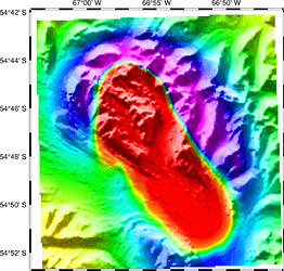
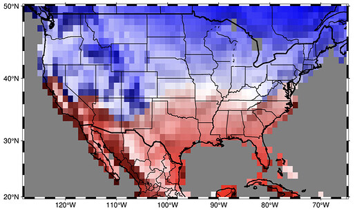
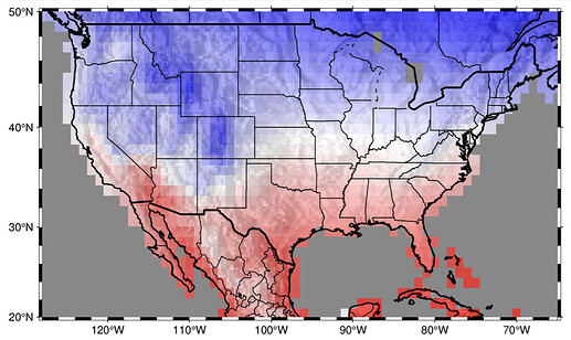
Grdimage with two datasets on top of each other

Hi,

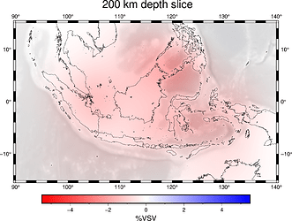
I am new to pygmt and would like to create a single figure with two datasets plotted on top of each other: transparent (or its gradient?) topography in the background plus an xarray.DataArray on top of it using a different colormap. My aim is a figure similar to this:
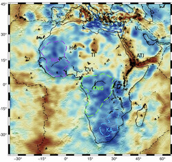
rsz_1goal

I was hoping to call grdimage twice – first for topography, and a second time for plotting the xarray.DatArray. But I can only make one of both work:
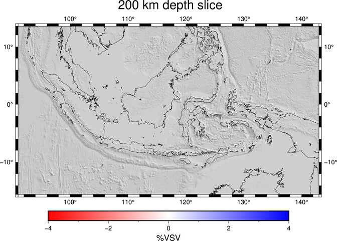
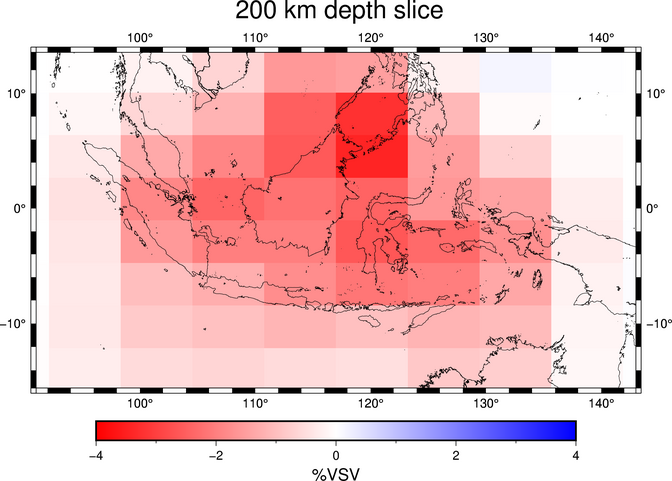
rsz_1grey_topo
rsz_vsv_figure

My code looks like this:

fig = pygmt.Figure()
proj = 'M8i'
param = "VSV"

### PLOT 1: TOPOGRAPHY ####

# create colorbar for topo
pygmt.makecpt(
    cmap='grayC', #temp 19lev
    series='-200000/40000/10000',
#    series='-40000/1000/1000',
    continuous=True,
    reverse=True,
)

fig.grdimage(
    grid=topo_data,
#    cmap="grayC", 
    region=[lon_min, lon_max, 
            lat_min, lat_max],
    projection=proj,
#     shading=True,
#     frame=True,
#    transparency=0.5,
    shading='+a45+nt0.5', #+a45+nt1
    )

### PLOT 2: VSV ####
# create colorbar for VSV
pygmt.makecpt(
    cmap='polar',
    series='-4/4/0.1',
    continuous=True,
    reverse=True,
)

## plot param values
 fig.grdimage(
     grid=ds, # xarray.DataArray containing VSV values
     region=[lon_min, lon_max, 
             lat_min, lat_max],
     projection=proj,
     cmap=True,
     frame=True,
     )

# plot coastlines
fig.coast(
    projection=proj,
    shorelines=True,
    )

# colorbar
colortext="+l\"%"+str(param)+"\""
fig.colorbar(frame=["af", colortext])
# set title
title="+t\" "+str(int(depth))+" km depth slice\""
fig.basemap(frame=["af", title])

fig.show(width=700)

Two questions:

  1. How can I combine both figures into one?
  2. Is there a better way of plotting the topography like this, that is is grdimage the best way forward here?

Thanks!
This sounds like a job for grdview. There is a drapegrid parameter in grdview that should allow you to overlay your xarray.DataArray grid on top of your topography. This might give you a start:

fig.grdview(
    grid=topo_data,
    drapegrid=ds,  # xarray.DataArray containing VSV values
    cmap=True, 
    region=[lon_min, lon_max, lat_min, lat_max],
    projection=proj,
    shading=True,
    frame=True,
)

You might also want to check out the surftype parameter. Usually I do surftype="sim" (for surface, image and mesh), but you might want to play around with the settings for your case. Note that grdview is typically used for 3D perspective plots of grids, but if you don’t use the perspective parameter, it should return a 2D flat map as with grdimage.

References:

Hi,

Thank you so much for your prompt reply! I’ve been faffing around with this for a while now and went through the tutorials you’ve attached (thank you, this was very helpful!) and was able to reproduce this.

I am not getting any further with my own example though. Please find my code below (fully reproducible, I hope):

import pygmt
import xarray as xr
import numpy as np

# setting up projection
proj = 'M8i'

# define region
lat_min, lat_max = -15., 15.
lon_min, lon_max = 90., 140.

# cut large topo file to region of interest
topo_data = '@earth_relief_10m' 
topo_data_SEA = pygmt.grdcut(topo_data,
                             region=[lon_min, lon_max, lat_min, lat_max],
                            )

# create xr.DataArray
size = 10
lat = np.linspace(start=lat_min, stop=lat_max, num=size)
lon = np.linspace(start=lon_min, stop=lon_max, num=size)
# create random data array in shape (lat,lon) 
data = np.random.randint(-5, 5, (size,size))

ds = xr.DataArray(data=data,
             dims= ["lat", "lon"],
             coords={"lat": lat,
                    "lon": lon})


# CREATE PLOT #

fig = pygmt.Figure()

#create colorbar for xarray.DataArray
pygmt.makecpt(
    cmap='polar',
    series='-5/5/0.5',
    continuous=True,
    reverse=True,
)

# plot
fig.grdview(
    grid=topo_data_SEA,
    drapegrid=ds,  # xarray.DataArray containing values to use for colormap
    cmap=True, 
    region=[lon_min, lon_max, lat_min, lat_max],
    projection=proj,
    shading=True,
    frame=True,
)

fig.show()

which produces the following output:

What is going wrong here?
My ds and topo_data_SEA look fine to me: both extend from lon_min to lon_max and lat_min to lat_max.

I’ve also had a look at the surftype option which works fine for this tutorial but my jupyter kernel will die if I add any of the available options.

Apologies for the late reply, I can reproduce your example map and the crash. I don’t have a proper solution yet, but noticed one thing you can fix first, that is, your ds xarray.DataArray had lat/lon flipped the wrong way around, it should be lon/lat instead (i.e. x/y):

ds = xr.DataArray(
    data=data,
    dims=["lat", "lon"],
    coords={
        "lon": lon,
        "lat": lat,
    },
)

Will still need to look into why the script is crashing. We had some problems with shading using xarray.DataArray grids crashing before (see https://github.com/GenericMappingTools/pygmt/issues/364) which I thought we fixed, but maybe there’s something with grdview that’s a bit buggy.

In the meantime, you could try:

  1. Save your ds to a NetCDF file and pass in a filename to drapegrid instead (i.e. using drapegrid="somefilename.nc"). Passing in filenames are a bit more stable than using xarray.DataArray grids
  2. Not sure if it matters, but have you tried making topo_data_SEA the same size as ds? Right now the shapes are (180, 300) and (10, 10) respectively.
  3. Try calling grdimage twice as you were trying before, but using transparency=50 for the second image (the one you want to overlay on top).

Sorry if this isn’t much help now, I’ll try and debug this a bit more over the weekend if I have time.

Hi,

Thanks for following up on this! I’ve changed lat and lon order – thanks for the hint! :slight_smile:

I’ve went through your suggestions, here are my results:

    1. Load xarray.DataArray from nc file (drapegrid=“ds.nc”) results in the following error:
grdview [ERROR]: Unknown grid format.
grdview (gmtapi_import_grid): Not a supported grid format [ds.nc]
[Session pygmt-session (6)]: Error returned from GMT API: GMT_GRID_READ_ERROR (18)
[Session pygmt-session (6)]: Error returned from GMT API: GMT_GRID_READ_ERROR (18)
psconvert [ERROR]: No hidden PS file /home/dw545/.gmt/sessions/gmt_session.128570/gmt_1.ps- found
 GMTCLibError: Module 'psconvert' failed with status code 78:
psconvert [ERROR]: No hidden PS file /home/dw545/.gmt/sessions/gmt_session.128570/gmt_1.ps- found 
    1. Get size for xarray.DataArray from size of topo_data_SEA, then try to use drapegrid="ds.nc" again:
grdview [ERROR]: Unknown grid format.
grdview (gmtapi_import_grid): Not a supported grid format [ds.nc]
[Session pygmt-session (18)]: Error returned from GMT API: GMT_GRID_READ_ERROR (18)
[Session pygmt-session (18)]: Error returned from GMT API: GMT_GRID_READ_ERROR (18)
psconvert [ERROR]: No hidden PS file /home/dw545/.gmt/sessions/gmt_session.129812/gmt_3.ps- found
 GMTCLibError: Module 'psconvert' failed with status code 78:
psconvert [ERROR]: No hidden PS file /home/dw545/.gmt/sessions/gmt_session.129812/gmt_3.ps- found 

When passing on the xarray.DataArray directly (drapegrid=ds with ds shape of (180, 300)), no error will be thrown and the following output will be generated:

    1. I’ve tried the transparency settings and while it does what I want, the problem is that I don’t. want to lose the colour intensity from the overlapping figure as this is the data I am actually interested it. I would just like the topography to be in the background, ideally its gradient as shown in the very first picture of this post.

Ok, I think I got it, or at least managed to a plot that didn’t crash. The key was to use fig.grdview(..., surftype="i", ...) where “i” means image in (see -Q option in grdview). The full code is as below:

Create topo and VSV data

import pygmt
import xarray as xr
import numpy as np

# setting up projection
proj = "M8i"

# define region
lat_min, lat_max = -15.0, 15.0
lon_min, lon_max = 90.0, 140.0

# cut large topo file to region of interest
topo_data = "@earth_relief_10m"
topo_data_SEA = pygmt.grdcut(
    topo_data,
    region=[lon_min, lon_max, lat_min, lat_max],
)

# create xr.DataArray
lat = np.linspace(start=lat_min, stop=lat_max, num=180)
lon = np.linspace(start=lon_min, stop=lon_max, num=300)
# create random data array in shape (lat,lon)
data = np.random.randint(-5, 5, size=(180, 300))

ds = xr.DataArray(
    data=data,
    dims=["lat", "lon"],
    coords={
        "lon": lon,
        "lat": lat,
    },
)
print(ds)

produces

<xarray.DataArray (lat: 180, lon: 300)>
array([[-4,  3, -1, ...,  3,  3,  0],
       [-3, -4, -5, ..., -2,  0,  1],
       [ 2,  3,  2, ...,  2,  0,  0],
       ...,
       [ 0, -1, -2, ...,  0, -3, -2],
       [-4,  3,  1, ...,  2,  2, -2],
       [-2, -5,  4, ...,  2, -1, -2]])
Coordinates:
  * lon      (lon) float64 90.0 90.17 90.33 90.5 ... 139.5 139.7 139.8 140.0
  * lat      (lat) float64 -15.0 -14.83 -14.66 -14.5 ... 14.5 14.66 14.83 15.0

Create grdview plot

fig = pygmt.Figure()

# create colorbar for xarray.DataArray
pygmt.makecpt(
    cmap="polar",
    series="-5/5/0.5",
    continuous=True,
    reverse=True,
)

# plot
fig.grdview(
    grid=topo_data_SEA,
    drapegrid=ds,  # xarray.DataArray containing values to use for colormap
    cmap=True,
    region=[lon_min, lon_max, lat_min, lat_max],
    projection=proj,
    surftype="i",
    shading=True,
    frame=True,
)

fig.show()

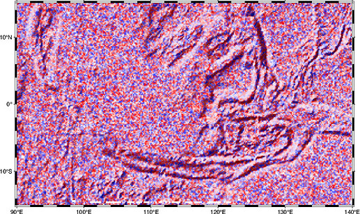
produces:

Hopefully your plot will look much better than the random data above. Let us know too if you need any help tweaking the plot!

1 Like

Hi, this looks great, thank you so much! I tried to reproduce this using exactly the same code you posted (literally copy pasted it and executed it in a new jupyter notebook). This will give me the following output:

rsz_output

Do you have idea why we cannot see the bathymetry here? I am on version 0.3.1 (further info below)

PyGMT information:
  version: v0.3.1
System information:
  python: 3.7.10 | packaged by conda-forge | (default, Feb 19 2021, 16:07:37)  [GCC 9.3.0]
  executable: /user/anaconda3/envs/salvus/bin/python
  machine: Linux-4.4.0-146-generic-x86_64-with-debian-stretch-sid
Dependency information:
  numpy: 1.20.2
  pandas: 1.2.4
  xarray: 0.17.0
  netCDF4: 1.5.6
  packaging: 20.9
  ghostscript: 9.53.3
  gmt: 6.1.1
GMT library information:
  binary dir: /user/anaconda3/envs/salvus/bin
  cores: 40
  grid layout: rows
  library path: /user/anaconda3/envs/salvus/lib/libgmt.so
  padding: 2
  plugin dir: /user/anaconda3/envs/salvus/lib/gmt/plugins
  share dir: /user/anaconda3/envs/salvus/share/gmt
  version: 6.1.1

Ah sorry, I was using the latest GMT 6.2.0rc1 instead of GMT 6.1.1 in the above. There were some problems with using grdview/grdimage from PyGMT in GMT 6.1.1 (see https://github.com/GenericMappingTools/pygmt/issues/1172 I think) that was fixed in GMT 6.2.0rc1. I’m able to reproduce your flat image on try-gmt (which uses PyGMT 0.3.1 and GMT 6.1.1).

If you don’t mind upgrading your GMT version to 6.2.0rc1 in Anaconda, you can do so using the following commands:

conda activate pygmt
conda install -y -c conda-forge/label/dev gmt==6.2.0rc1
conda list  # check that GMT 6.2.0rc1 is installed

Hopefully things will finally work for you then!

I also have done the same with grdview. I wonder if this would be a good feature request for grdimage. In my case with grdimage I often had to resample the grid which grdview handle without any problem. Now I am using grdview directly but I don’t know if would be better if the same machinery is available directly for grdimage.

Just so I understand what is being asked here of grdimage: You would like to derive the intensities from one grid (say topo) and look up the colors via the CPT and another grid, and the two grids may not have the same grid spacing? It would seem this would require a modification to the grdimage -I option to allow you to pass a grid there that is not an intensity grid but a surface from which you wish to derive intensities (instead of from the main grid).

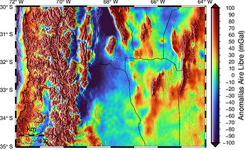
Yes, basically that. For example I made this figure with the following commands:

gmt grdgradient $DEM -A270 -G$SHADOW -Ne0.8
gmt grdsample $FAA -G$CUT -R$SHADOW
gmt grdimage -R -J -O -K $CUT -C$color >> $OUT -I$SHADOW

Also it would be good to be able to use “irregular” grids. In this case I made it with grdview.

gmt grdgradient %DEM% -A0/270 -G%SHADOW% -Nt1.2
gmt grdview -R -J -O -K %DEM% -C%color% -Qc -JZ1c -I%SHADOW% -p180/90 -G%MAG% >> %OUT%
1 Like

So what do you think? Should I open a feature request?

Yes, please do - it should not be too difficult I think.

1 Like

Hi @pwessel and @Esteban82! Following up on this modification request to grdimage… Is it now possible to use different grid spacings for the underlying topo grid and the overlying CPT grid? Thank you!

Yes, I think that it should work if you use GMT 6.4 or the Dev version.

Just to clarify - do you mean the dev version of PyGMT? I updated to PyGMT v0.7.0 with GMT 6.4.0 dependency but I’m still receiving the error “grdimage [ERROR]: Dimensions of intensity grid do not match that of the data grid!” when testing the process (code below).

fig = pygmt.Figure()
with pygmt.config(MAP_ANNOT_OFFSET_PRIMARY=‘0.1c’):
fig.basemap(frame=[‘af’], region=[-128, -65, 20, 50], projection=‘M6i’)
fig.coast(area_thresh=‘100000’,water=‘gray62’)

pygmt.grdgradient(grid = pygmt.datasets.load_earth_relief(resolution=‘01d’, region=[-128, -65, 20, 50], registration=“gridline”, use_srtm=False), azimuth=0/270,outgrid=‘SHADOW’,normalize=‘t1.2’)

fig.grdimage(grid=‘climate.nc’, cmap=‘polar’, shading=‘SHADOW’)
with pygmt.config(PS_LINE_CAP=‘round’, PS_LINE_JOIN=‘round’):
fig.coast(resolution=‘h’, borders=[‘1/1.5p’, ‘2/0.5p’], shorelines=‘1/1’,area_thresh=‘500’)

I would love to use 30m or 15m resolution of the earth relief dataset while keeping a 1° by 1° CPT grid. If it’s as simple as waiting for the next PyGMT release, that’s fantastic.

You probably can do this :

  • grdimage @relief
  • coast (to clip)
  • grdimage climate.nc -Ccolor.cpt -t75 (for transparency)

Like this you have the relief at whatever resolution, climate.nc at its native resolution with semi-transparent color encompassed within coast boundary

1 Like

Thank you @PlanetGus! That is much closer to what I am envisioning.