How can I clip features (e.g. Rivers) to a smaller region than that map region?

I have a map for a specific region

fig.coast(
    # Set the x-range from 10E to 20E and the y-range to 35N to 45N
    region='-6.061164/2.790309/48/57',
    ...
)

I want to add a specific river (the Trent river) that is bound by -2.062697/0.214867/52.737217/53.791475 to the map, but using that rectangle as the region for another call to coast makes the river occupy the whole page.

fig.coast(
    region='-2.062697/0.214867/52.737217/53.791475',
    rivers='3/2p,blue,solid',
)

Is there a way to “clip” features without using the region specifier?

Please, post this in the PyGMT category.

This isn’t so much a question about PyGMT. For the most part, the Python is just a more readable wrapper around the standard GMT. I posted Python because that’s what I’m using and I wanted to provide some meaningful example, rather than coming up with pscoast commands that I wasn’t using and would probably be incorrect.

The question is one of GMT behavior. Given a particular region for the map, how can I select only features in a given sub-region. Say, I want to color different major rivers in the main region different colors. How could I use different pscoast commands to select only rivers in a given rectangle (a smaller rectangle than the region used for the map)?

Only (as I’m seeing it now) if you manage to dump the data in the subregion of interest and plot it again with plot.

One apparent possibility is to use clip, the other to dump data using coast -M
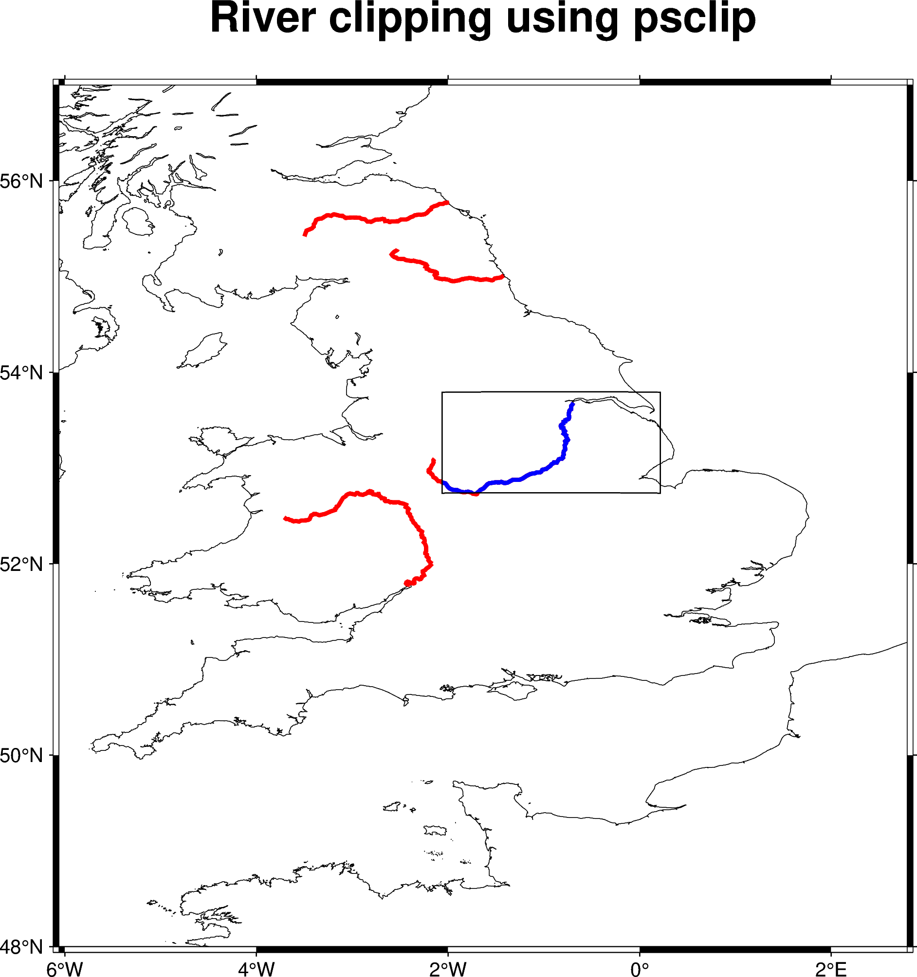
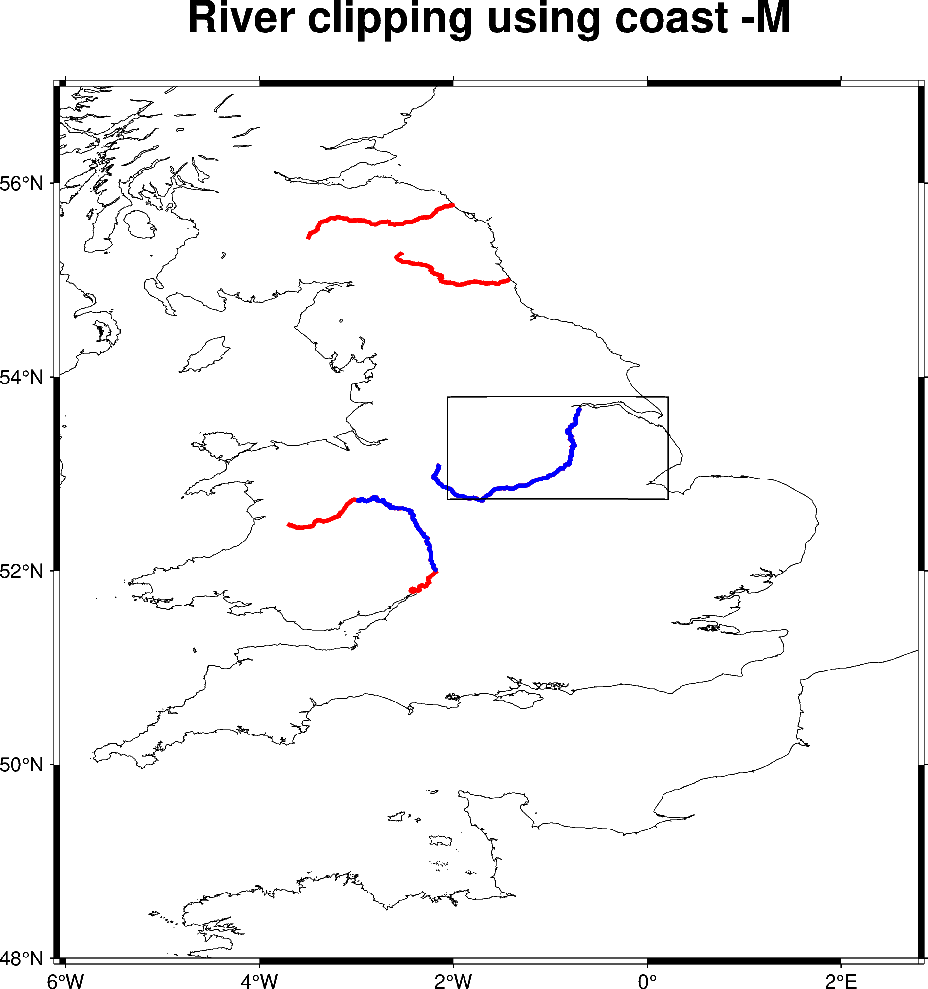
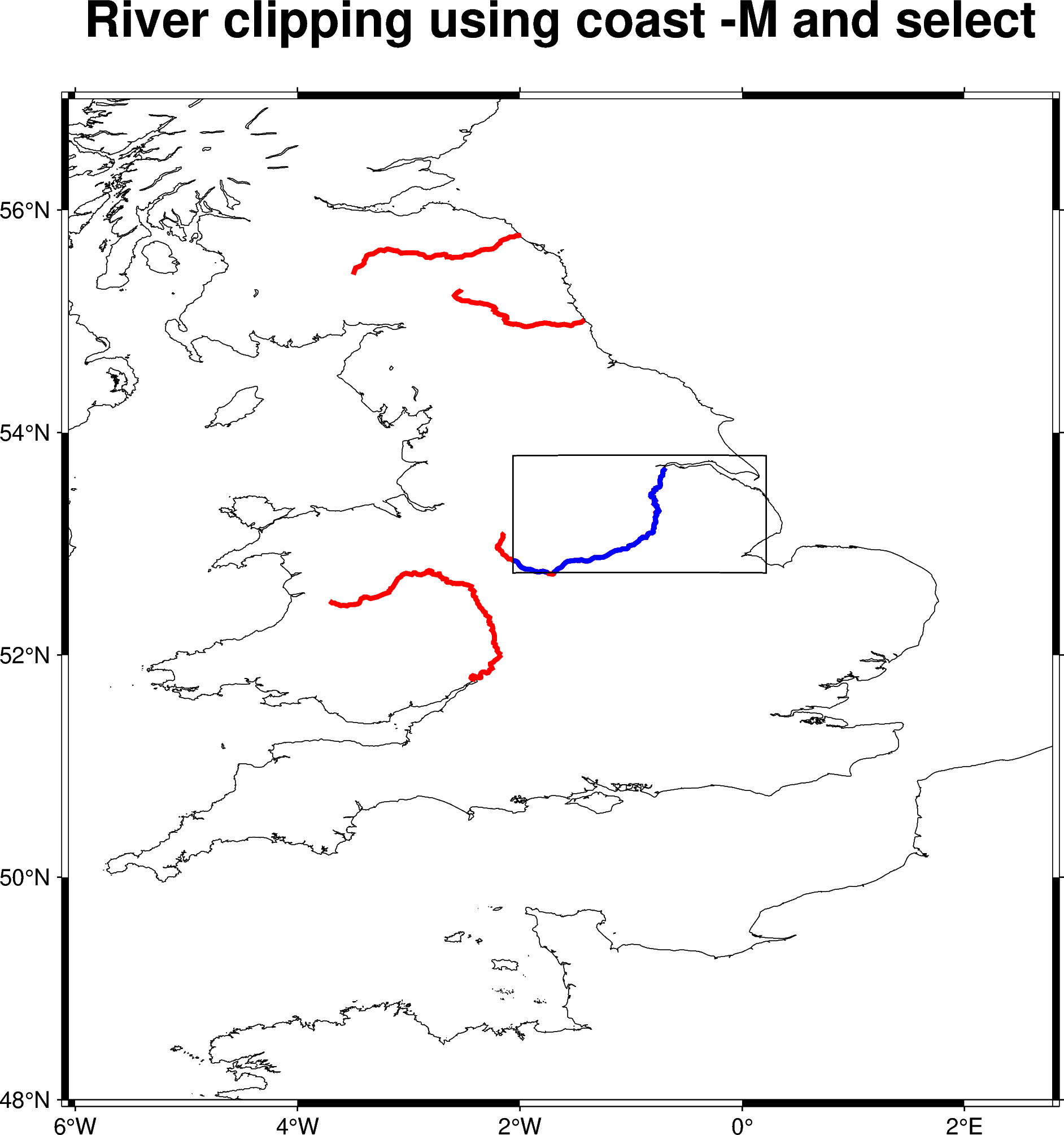
Neither appears to be wrapped by pygmt as far as I can understand. I tried using both using GMT C API calls mechanism provided by pygmt, just out of curiosity. clip does the job precisely but the result looks ugly as clip clips the graphic representation which does not look good if rivers were plotted using a thick pen. coast however dumped an extra river segment quite far outside the specified -R... boundaries which does not look too good either. See some spagetti code and the plots below. Blue line shows rivers clipped out by the corresponding method. Red line shows all level 3 rivers -I3/2p,blue,solid as specified by the topic started. Why does coast behave so? Thanks!

using psclip:

import pygmt

XMIN=-2.062697; XMAX=0.214867; YMIN=52.737217; YMAX=53.791475
clipping_rectangle=f'{XMIN} {YMIN}\n{XMIN} {YMAX}\n{XMAX} {YMAX}\n{XMAX} {YMIN}\n{XMIN} {YMIN}\n'
clipping_rectangle_file = 'clipping_rectangle.txt'

with open(clipping_rectangle_file,"w") as f:
    f.write(clipping_rectangle)

fig = pygmt.Figure()

region = '-6.061164/2.790309/48/57'
title = 'River clipping using psclip'
fig.coast(
    region=region,
    shorelines=True,
    rivers='3/2p,red,solid',
    frame=[f'WSen+t{title}',"xa","ya"]
)

# equivalent to
# gmt clip -R-2.062697/0.214867/52.737217/53.791475 clipping_rectangle.txt
with pygmt.clib.Session() as s:
    # Initialize clipping
    args = [f'{clipping_rectangle_file}', f'-R{region}']
    s.call_module('clip', args=' '.join(args))

fig.coast(
    #region='-2.062697/0.214867/52.737217/53.791475',
    rivers='3/2p,blue,solid',
)

with pygmt.clib.Session() as s:
    # Finalize clipping
    s.call_module('clip', args='-C1')

fig.plot(
    region=region,
    data=clipping_rectangle_file,
    pen='0.5p,black,solid'
)

fig.savefig("clipping_pygmt_1.png", show=True)

using coast -M:

import pygmt

XMIN=-2.062697; XMAX=0.214867; YMIN=52.737217; YMAX=53.791475
clipping_rectangle=f"{XMIN} {YMIN}\n{XMIN} {YMAX}\n{XMAX} {YMAX}\n{XMAX} {YMIN}\n{XMIN} {YMIN}\n"
clipping_rectangle_file = 'clipping_rectangle.txt'

with open(clipping_rectangle_file,"w") as f:
    f.write(clipping_rectangle)

fig = pygmt.Figure()

region='-6.061164/2.790309/48/57'
title = 'River clipping using coast -M'
fig.coast(
    region=region,
    shorelines=True,
    rivers='3/2p,red,solid',
    frame=[f'WSen+t{title}',"xa","ya"]
)

region1 = '-2.062697/0.214867/52.737217/53.791475'
clipped_river_file = 'clipped_river_file.txt'

# equivalent to
# gmt coast -R-2.062697/0.214867/52.737217/53.791475 -M -I3 > clipped_river_file.txt
with pygmt.clib.Session() as s:
    args = [f'-R{region1}', '-M', '-I3', f'> {clipped_river_file}']
    s.call_module('coast', args=' '.join(args))

fig.plot(
    region=region,
    data=clipped_river_file,
    pen='2p,blue,solid'
)

fig.plot(
    region=region,
    data=clipping_rectangle_file,
    pen='0.5p,black,solid'
)

fig.savefig("clipping_pygmt_2.png", show=True)

If I run coast -M output through select, the result looks like what I expected to see (also suboptimal choice of clipping rectangle becomes obvious). More spagetti and a plot:

import pygmt

XMIN=-2.062697; XMAX=0.214867; YMIN=52.737217; YMAX=53.791475
clipping_rectangle=f"{XMIN} {YMIN}\n{XMIN} {YMAX}\n{XMAX} {YMAX}\n{XMAX} {YMIN}\n{XMIN} {YMIN}\n"
clipping_rectangle_file = 'clipping_rectangle.txt'

with open(clipping_rectangle_file,"w") as f:
    f.write(clipping_rectangle)

fig = pygmt.Figure()

region='-6.061164/2.790309/48/57'
title = 'River clipping using coast -M and select'
fig.coast(
    region=region,
    shorelines=True,
    rivers='3/2p,red,solid',
    frame=[f'WSen+t{title}',"xa","ya"]
)

region1 = '-2.062697/0.214867/52.737217/53.791475'
clipped_river_file = 'clipped_river_file.txt'

# equivalent to
# gmt coast -R-2.062697/0.214867/52.737217/53.791475 -M -I3 > clipped_river_file.txt
with pygmt.clib.Session() as s:
    args = [f'-R{region1}', '-M', '-I3', f'> {clipped_river_file}']
    s.call_module('coast', args=' '.join(args))

outfile = 'out.txt'
pygmt.select(data=clipped_river_file, region=region1, output_type='file', outfile=outfile)

fig.plot(
    region=region,
    data=outfile,
    pen='2p,blue,solid'
)

fig.plot(
    region=region,
    data=clipping_rectangle_file,
    pen='0.5p,black,solid'
)

fig.savefig("clipping_pygmt_3.png", show=True)