Yeap, but no need. GMT can do it directly as I shown in my ~first answer.
Well, I did say I was a dinosaur. That grdconvert feature wasn’t in GMT3! Good one to know.
Just beware, the resulting grid provides lunar radius values.
And another thing to be aware of. There are some processing artifacts hidden among the details in those DEM files.
Right, easy to let go unnoticed
SPHEROID["unknown",1737400,0]],
I’ve been on a journey with this LRO data.
Tried a bunch of things. Ultimately what worked was:
- Download OSGeo4W which installs GDAL.
- open OSGeo4W and run the following one-line command to make a .nc file that pygmt can open:
gdal_translate C:\Users\_me_\PycharmProjects\LunarSouthPoleLRO\LROData\ldem_80s_80m\float_img\ldem_80s_80m_float.lbl C:\Users\_me_\PycharmProjects\LunarSouthPoleLRO\LROData\ldem_80s_80m\float_img\ldem_80s_80m_float.nc
- Run this in Python:
import pygmt
import os
filepath = r"C:\Users\_me_\PycharmProjects\LunarSouthPoleLRO\LROData\ldem_80s_20m\float_img\ldem_80s_20m_float.nc"
savepath = r"C:\Users\_me_\PycharmProjects\LunarSouthPoleLRO\pyGMTfigures\ldem_80s_20m\ldem_80s_20m_float_nc.png"
fig = pygmt.Figure()
# noinspection PyUnresolvedReferences
fig.grdimage(filepath)
fig.show()
fig.savefig(savepath)
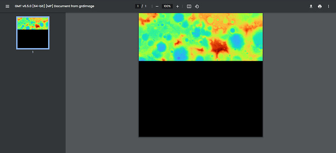
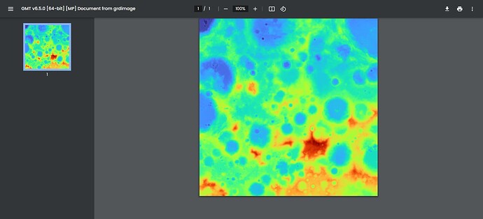
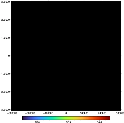
Important to note that pyGMT cannot display the 20m data in the browser, it can only load part of it before failing and displaying the rest of the map as black. The lower resolution 80m data can be displayed in the browser. The figure you get for the 20m data from:
fig.savefig(savepath)
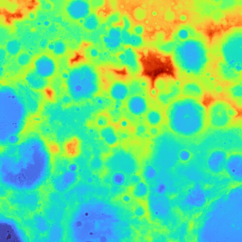
looks perfectly fine though, again pyGMT just cannot display a figure that big in the browser. Idk if its pyGMT, GMT, my computer, the browser, or some combination thereof, but it does not work. It saves perfectly fine though. Here is what the browser displays for the 20m data:
Here is the saved figure for the 20m data:
If you tried this with the 80m data it would both display and save fine though.
Now on to what did not work. The .tif file method did not work well for me:
I ran the following commands in GDAL to make a .tif file from the LRO data.
gdal_translate -of GTiff C:\Users\_me_\PycharmProjects\LunarSouthPoleLRO\LROData\ldem_80s_20m\float_img\ldem_80s_20m_float.lbl C:\Users\_me_\PycharmProjects\LunarSouthPoleLRO\LROData\ldem_80s_20m\float_img\ldem_80s_20m_float.tif
Using pyGMT to read from this .tif file:
import pygmt
import osfilepath = r"C:\Users\_me_\PycharmProjects\LunarSouthPoleLRO\LROData\ldem_80s_80m\float_img\ldem_80s_80m_float.tif"
savepath = r"C:\Users\_me_\PycharmProjects\LunarSouthPoleLRO\pyGMTfigures\ldem_80s_80m\ldem_80s_80m_float_tif.png"
fig = pygmt.Figure()
# noinspection PyUnresolvedReferences
fig.grdimage(filepath)
fig.show()
fig.savefig(savepath)
This displayed a giant black square and also saved a giant black square as a file.
Now if I made the .tif file in python using the GDAL module itself, I got something different. This is the code I used to make the .tif file in Python with GDAL:
from osgeo import gdal
import ososCWD = os.getcwd()
data_path = r"\LROData\ldem_80s_80m\float_img\ldem_80s_80m_float.lbl"
ds = gdal.Open(osCWD+data_path)
gt = ds.GetGeoTransform()
proj = ds.GetProjection()
band = ds.GetRasterBand(1)array = band.ReadAsArray()
driver = gdal.GetDriverByName(‘GTiff’)outds = driver.Create(
osCWD+data_path.replace(‘lbl’, ‘tif’),
xsize=array.shape[1],
ysize=array.shape[0],
bands=1,
eType=gdal.GDT_Float32
)outds.SetGeoTransform(gt)
outds.SetProjection(proj)
outband = outds.GetRasterBand(1)
outband.WriteArray(array)
outband.SetNoDataValue(np.nan)
outband.FlushCache()outband = None
outds = Nonefig = pygmt.Figure()
fig.grdimage(osCWD+data_path.replace(‘lbl’, ‘tif’)) # open the .tif file just made.
fig.show()
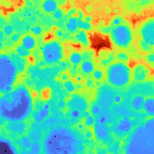
This works, for the most part. The map has a white spot the upper right quadrant within the dark red area and a few small black spots in the very bottom very left of the map. These white and black spots were pure white and pure black, and not part of the general color pallet of the map. Here’s the figure so you can see yourself:
The .tif file made from gdal_translate did not work in pyGMT, the tif file made in Python using the gdal module did work.
What also worked was using gdal to read the data and then passing that into matplotlib. Here is the code for that:
from osgeo import gdal
import matplotlib.pyplot as plt
import ososCWD = os.getcwd()
data_path = r"\LROData\ldem_80s_20m\float_img\ldem_80s_20m_float.lbl"ds = gdal.Open(osCWD+data_path)
gt = ds.GetGeoTransform()
proj = ds.GetProjection()band = ds.GetRasterBand(1)
array = band.ReadAsArray()plt.figure() # Plot in matplotlib
plt.imshow(array)
plt.show()
Matplotlib works perfectly when using the .tif file created with the gdal_translate command in OSGeo4W. It also works with the .tif file made using the gdal module in Python in the way I showed above. matplotlib can also plot the .tif if you give it an array made by reading the .lbl NASA file into the gdal module. Matplotlib works with both sizes (80m and 20m resolution) aswell, with no issue. I haven’t tried the .nc files in matplotlib, but I don’t think I need to as they work with pyGMT and that is what I am using.
Shame matplotlib was a bit more user friendly though. It worked with the original NASA data through gdal, as well as both ways of making .tif files through the gdal module and the gdal_translate command.
Last thing to note:
Interestingly, loading the .lbl file through gdal and then converting it to an array and using xarray and passing that into pyGMT works to plot a figure, but it comes out upsidedown! There is no white spot from this method that results from loading the .tif file made through the gdal module directly though. Here’s the rest of the code and the resulting figure for that:
# Just make the xarray and pass that to pyGMT
import xarray as xr
# get the array using gdal to read the .lbl file from the previous code & make an array
data_xarray = xr.DataArray(array)
fig = pygmt.Figure()
# noinspection PyUnresolvedReferences
fig.grdimage(grid=data_xarray)
fig.show()
All in all this is what works for pygmt:
First in OSGeo4W:
gdal_translate C:\path\file.lbl C:\path\file.nc
Then in Python:
import pygmt
fig = pygmt.Figure()
fig.grdimage(C:\path\file.nc)
fig.show()
fig.savefig(C:\path\file.png)
-
I did not have any luck with the .tif files in pyGMT. They either came out all black if made through gdal_translate, or with white/black blobs if made through the Python gdal module.
-
loading the .lbl file into python with gdal, turning that data into an xarray, and then passing it to pygmt plots the map, just upsidedown.
-
matplotlib works with .lbl files and .tif files read with the gdal module. The .tif files can be made either through gdal_translate in OSGeo4W or in Python with the gdal module, they will work either way.
played with the file, got the same black square
gmt grdimage ldem_80s_20m_float.xml -BWSen -Bxa -Bya -png ldem_80s_20m_float.xml
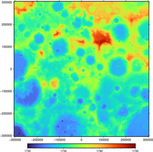
automatic color scale/range seems off by x2, so the square is black. The real scale is approx 1730…1745:
$ gmt grdinfo ldem_80s_20m_float.xml
ldem_80s_20m_float.xml: Title: Grid imported via GDAL
ldem_80s_20m_float.xml: Command:
ldem_80s_20m_float.xml: Remark:
ldem_80s_20m_float.xml: Gridline node registration used [Cartesian grid]
ldem_80s_20m_float.xml: Grid file format: gd = Import/export through GDAL
ldem_80s_20m_float.xml: x_min: -303990 x_max: 303990 x_inc: 20 name: x n_columns: 30400
ldem_80s_20m_float.xml: y_min: -303990 y_max: 303990 y_inc: 20 name: y n_rows: 30400
ldem_80s_20m_float.xml: v_min: 1730.21968927 v_max: 1744.30686321 name: z
ldem_80s_20m_float.xml: scale_factor: 1 add_offset: 1737.4 packed z-range: [-7.18031072617,6.90686321259]
ldem_80s_20m_float.xml: Default CPT:
+proj=stere +lat_0=-90 +lat_ts=-90 +lon_0=0 +x_0=0 +y_0=0 +R=1737400 +units=m +no_defs
manual palette setting works:
gmt makecpt -Cturbo -T1730/1745 > ldem_turbo.cpt
gmt grdimage ldem_80s_20m_float.xml -BWSen -Bxa -Bya -png ldem_80s_20m_float -Cldem_turbo.cpt
