How to properly georeference an irregular (Lambert conformal) grid using pygmt

I’m starting a transition from regular GMT to pygmt and and I’m having problems to plot data fields in grib format due to wrong georeferentiation.

I’m working a simple grib file with a single “message”. Note that the grid is irregular, in particular it is Lambert conformal. Now, I open it with xarray (which I assume is the format preferred by pygmt???).

import pygmt
import xarray as xr
import numpy as np
grb = xr.open_dataset('class_thun_m_000_0112.grb')

The result looks more or less good. There is some metadata a bit funny with unnecessary coordinates and some attributes not well digested by GMT when I try to plot it (probably because the file itself is not perfectly formed). But anyway, I’m just interested in the metadata related to georeferentiation. Therefore, and to make sure I control de values of the field, I have made up random data and taken just the coordinates from the original grib file to create a fresh new DataArray.

coords = grb['unknown'].coords
values = np.random.randn(*grb.shape)

grid = xarray.DataArray(values, coords=coords)
grid.name = 'random'

Now, when I try to plot this with the following code:

fig = pygmt.Figure()
fig.basemap(region=[-20, 20, -10, 60], projection="M15c", frame=True)
fig.coast(shorelines=["1/1p,black"], land='green', water='skyblue')
fig.grdcontour(grid=grid)
fig.show()

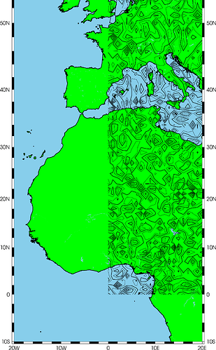
I get this image, which clearly shows that gmt is not aware of the actual coordinates (the data covers the Iberian Peninsula). Instead, it is erroneously interpreting the array index as degrees.

How can I make GMT correctly understand the georeferentiation? Can I work with non-regular grids anyway? In the old good times of regular GMT, to cope with this type of grids I had to make an overlay, plotting the coasts with the actual projection, and then overlaying the grid using X projection. Something like this classical example. Is it possible to translate this approach to pygmt?
Whether you using GMT CLI or a wrapper, GMT still requires you to regard any irregular grids before they can be plotted. Basically, get the list of x, y, z points and use blockmean, surface or similar to create a regular grid.

I have zero experience with grib files but it looks like GDAL has some complains on yours.

Loading your grib file from Julia

# many complains
...
Warning 1: GRIB: Parameter 140 is > 127, so it falls in the local use section of
the parameter table (and is undefined on the international table.> 
Using default for now(which might lead to erroneous interpretation), but please email arthur.taylor@noaa.gov
about adding this table to his 'degrib1.c' and 'grib1tab.c' files.

G = gmtread("class_thun_m_000_0112.grb", grid=true, gdal=true);

but there is only one array in that file that seems a regular grid, which plots this (whatever it is)

imshow(G, coast=(shore=:white,), colorbar=true)

Thanks for the replies. Before answering I wanted to try different things. Eventually, I had to re-learn GMT from Python, which is why it took me so long to reply.

@Joaquim, this grib raises various warnings because it does not fulfill every convention about variable names, tables and so on. I’m also not an expert in grib, but I’m pretty sure it is not really the issue here. The data is storm classification in weather forecasting, by the way.

Anyway I was finally able to “crop” the funny metadata and work with the raw data. Doing this and overlying images in two coordinates systems, the actual one (lambert) and a XY one with a region carefully crafted, I was able to recreate the figure I wanted. I’d like to avoid the interpolation solution to avoid losing data, but specially to minimise computational overheads. It would be silly to interpolate to a regular grid, and then to interpolate again to plot using the original grid. Or did I miss your point @pwessel?

However, I’m now puzzled and curious how @Joaquim was able to get that image. Somehow it seems that Julia understood the georefence metadata? And you were able to plot it out of the box!? Doesn’t this conflict with the argument of Paul about GMT not handling irregular grids?

Julia is only calling GMT, that calls GDAL to read that grid, which is a regular grid.
I guess you should obtain the same by doing (and plot it after).

gmt grdconvert class_thun_m_000_0112.grb=gd -Gclass_thun_m_000_0112.grd