Great! I can re-produce the figure. Thank you.
Let’s check the data structure.
ncdump RDEFT4_20101021.nc | head -200
netcdf RDEFT4_20101021 {
dimensions:
x = 304 ;
y = 448 ;
variables:
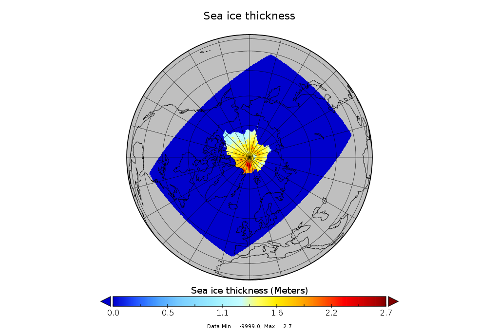
float sea_ice_thickness(y, x) ;
sea_ice_thickness:units = "Meters" ;
sea_ice_thickness:long_name = "Sea ice thickness" ;
float snow_depth(y, x) ;
snow_depth:units = "Meters" ;
snow_depth:long_name = "Snow depth" ;
float snow_density(y, x) ;
snow_density:units = "Kg / Meters^3" ;
snow_density:long_name = "Snow density" ;
float lat(y, x) ;
lat:units = "Degrees" ;
lat:long_name = "Latitude" ;
float lon(y, x) ;
lon:units = "Degrees" ;
lon:long_name = "Longitude" ;
float freeboard(y, x) ;
freeboard:units = "Meters" ;
freeboard:long_name = "Ice freeboard" ;
float roughness(y, x) ;
roughness:units = "Meters" ;
roughness:long_name = "Ice surface roughness" ;
float ice_con(y, x) ;
ice_con:units = "Percent x 100" ;
ice_con:long_name = "Sea ice concentration" ;
// global attributes:
:Title = "CryoSat-2 sea ice thickness and ancillary data" ;
:Abstract = "This data set contains monthly averaged Arctic sea ice thickness estimates and ancillary data. The primary data set used in the production of these data come from the ESA CryoSat-2 satellite. Sea ice freeboard is determined from CryoSat-2 using the method described in the Reference section below. In brief, this method uses a physical model to determine the best fit to each CryoSat-2 waveform.The fitted waveform is used to determine the retracking correction and also allows determination of the surface roughness within the footprint. For sea ice floes, the dominant backscattering layer is taken to be from the sea ice surface and thus sea ice freeboard is here defined as the height of the ice layer above the local sea surface. The DTU10 MSS is subtracted from each elevation measurement and the elevations from leads and sea ice floes are placed onto a 25 km polar stereographic grid. Sea ice freeboard is then determined by subtracting the gridded sea surface elevation from the gridded sea ice floe elevation. Snow depth is constructed from a modified Warren climatology of snow depth on sea ice. Sea ice thickness is retrieved assuming hydrostatic balance and nominal densities of snow, ice, and water. Retrievals are only done when the sea ice concentration is at least 70%. Sea ice concentration is from the near real time DMSP SSMI_S daily polar gridded data set with the pole hole set to a constant value of 100%." ;
:Projection = "CryoSat-2 elevation data have a nominal footprint size of 380 m x 1,650 m and are referenced to the WGS-84 ellipsoid. The derived CryoSat-2 freeboard data, and all ancillary data, have been gridded to the 25 km polar stereographic SSM/I grid. The center latitude and longitude for each grid point are provided with the data." ;
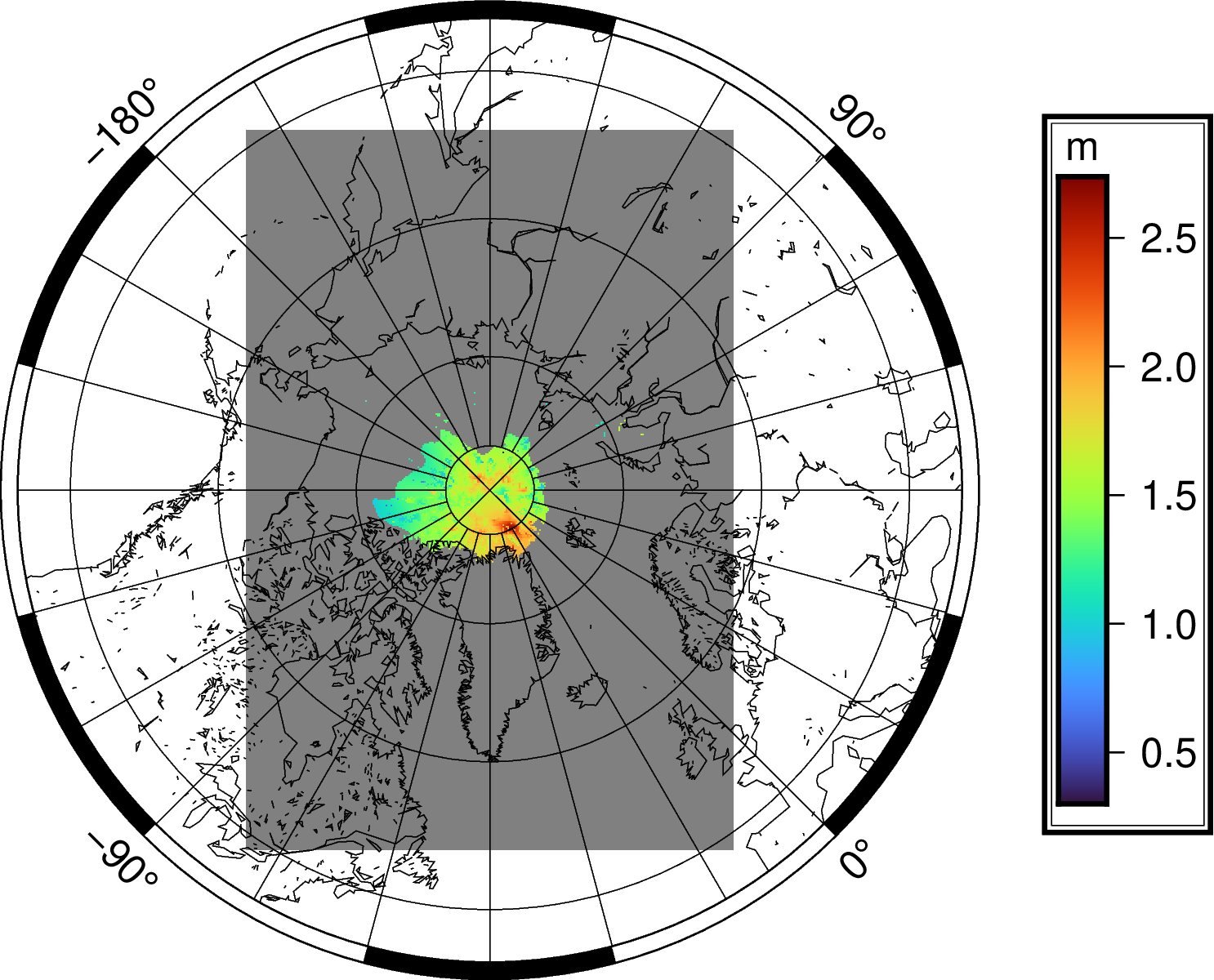
We find that the x and y values are just the index of the two dimensions. They are not the projected coordinates in the Polar Stereographic projection and their unit is not meter (just index).
The lat and lon are stored in the variables as with index of (y,x). As we dump the variables using grd2xyz, the true value of the latitude and longitude could be seen. However, the geo-coordinates not in regular grid nodes.
The GMT can not plot this kind of data directly because of the special data structure. GMT can not read the true coordinate no matter the geo or xy forms.
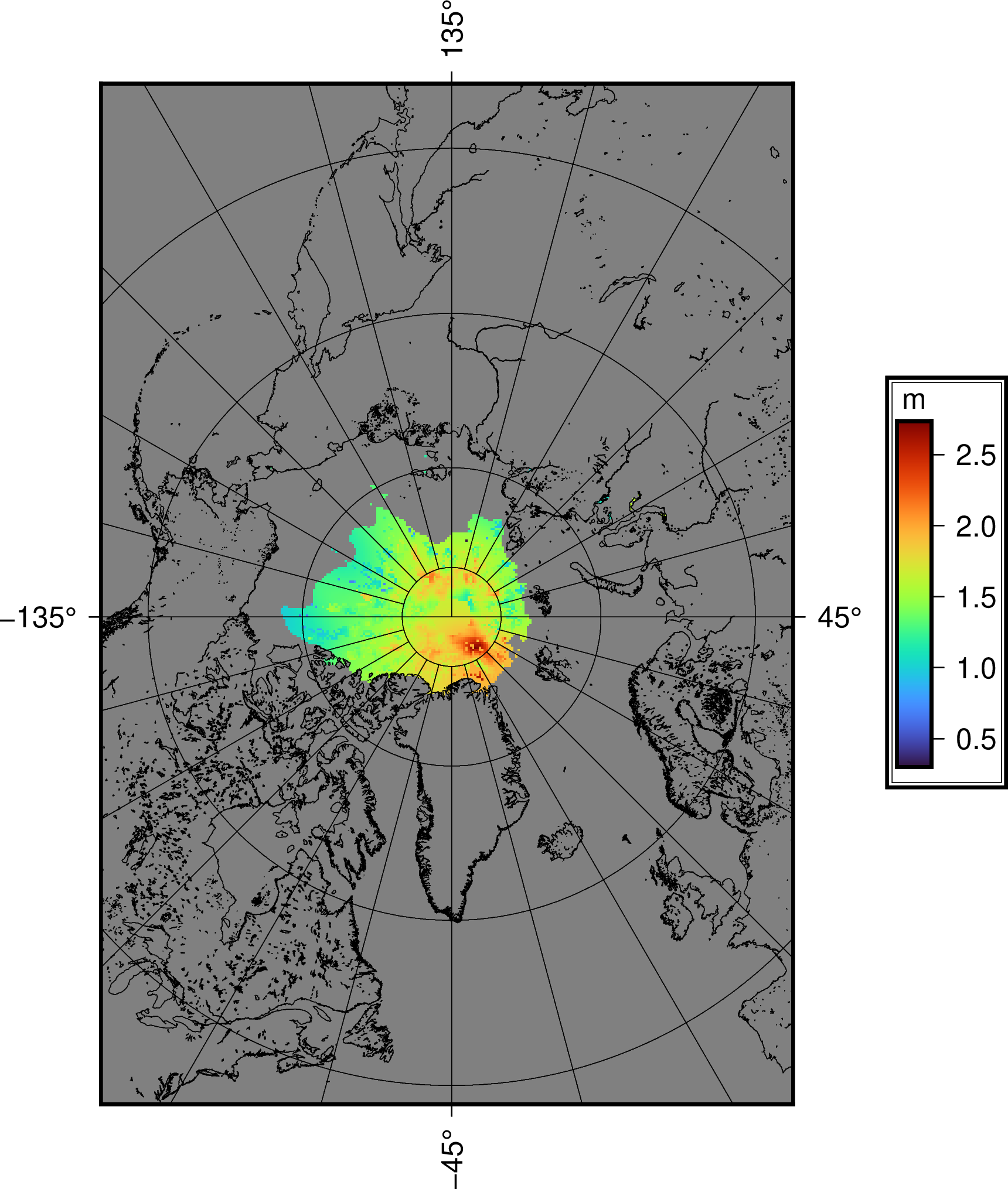
After a coordinates transform as adopted by mkononets, the data can be plotted.
So, maybe the GMT developers could consider adding a new feature about this. It will be very useful to plot this projection which is widely used in polar area.