I’ve been building a personal website with weather products for the Tonga region which heavily use GMT. The website is here: https://met.nomuka.com None of the maps or plots are anything particularly fancy, but I thought maybe some others would be interested.
Satellite Image
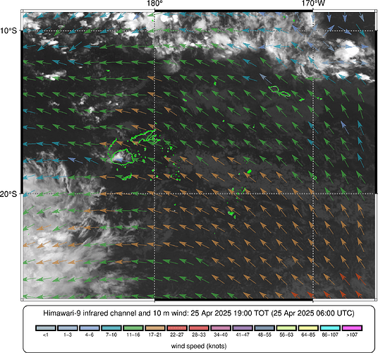
This image starts its life as a JPEG image on the Japan Meteorological Agency website. I know the map projection they are using, so to convert it to a GMT grd file I use the netpbm tools to convert it to a Sun raster image, and then use grdconvert to make it into a NetCDF file which can then be manipulated with other GMT tools. Then wind vector data from the European Centre for Medium Range Weather forecasts are overlaid on the satellite image as coloured arrows, where the colours are in a colour palette based on the Beaufort wind speed scale.
Observations time series
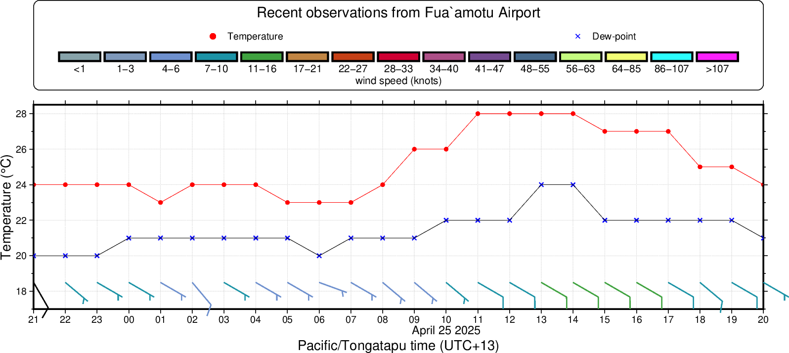
These data start life as coded messages from the Tonga Meteorological Services in a format known as METAR. These are decoded using various regular expressions, and plotted as time series. I use the Beaufort colour palette to colorise wind barbs created using the GMT barb command.
ECMWF weather charts
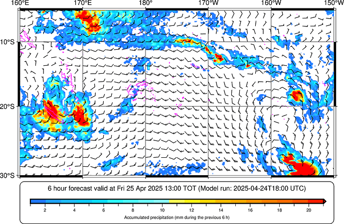
These simply show accumulated rainfall and wind for the Southwest Pacific. Data are from ECMWF. I wanted to simply use one of the many graphics that ECMWF put on their website, but none focussed in on the Southwest Pacific region, so once again GMT came to the rescue.
7 Likes
Neat 
Could you share the scripts you used too ?
Nice. And about the first fig, you mean you ended up with nc grid of RGB’s in uint8, or floats? Wouldn’t grdimage -Dr have worked for making the base image?
Yes, initially I simply put the images in using grdimage. And that worked fine, even when map projections were changed. But then I wanted to manipulate the images:
- Remove a date stamp on the image (and move it to the legend)
- Various experiments with applying colour palettes.
So I wanted to get the JPEG into a NetCDF file, and the only way I could easily see how to do this was via an 8-bit Sun raster image. Here’s the code:
wget "${sat_server}/${sat_file}" -O - | jpegtopnm - | ppmtopgm | pnmtorast -standard - > ${tmpdir}/sat.sun

gmt grdconvert ${tmpdir}/sat.sun=rb -G${tmpdir}/sat.nc
It’s a bit gross (that format dates from the 1980s I believe), but it works.
The scripts have a lot of site-specific stuff in them. If there are particular parts of them that you are interested in, I’m happy to post it here.
I think just the actual plotting part. It could be of use for a tutorial @Esteban82 is developping 
These may not be the most beautiful GMT scripts - they’re still a work in progress.
Plot satellite picture with wind vectors
gmt begin ${www_dir}/${sat_img} PNG E 72 -C
        gmt set GMT_THEME modern
        gmt set PROJ_LENGTH_UNIT c
        gmt basemap -JM15c \
                -R${map_west}/${map_south_cut}/${map_east}/${map_north}+r -BWseN \
                -Bpxa10 -Bpya10
        gmt grd2cpt ${tmpdir}/cutsat.nc -Cgray -T0/255/1
        gmt grdimage ${tmpdir}/cutsat.nc
        gmt coast -Dh -Wthinnest,green
        gmt grdvector ${tmpdir}/ecmwf.nc?u10+s1.94384 \
                ${tmpdir}/ecmwf.nc?v10+s1.94384 -Ix4 \
                -Sl1.5c -Q+e+h0.5+jc -C${tmpdir}/beaufort.cpt  -Wthinner+c -t30
        gmt legend -DjBL+w15c+jTL+o0/0.3 -F+pthinner,black+r <<- END
        H 9,Helvetica,black ${title}
        G 1l
        B ${tmpdir}/beaufort.cpt 0.5 0.2 --FONT_ANNOT_PRIMARY=6,Helvetica,black -L0.1 -S+c
        L 8,Helvetica,black C wind speed (knots)
        END
gmt end
Plot observations
gmt begin /var/www/html/obs/obs_nftf PNG E150 -C
        region=$(gmt info -I3600/1+R0/0/3/0.5 ${tmpdir}/tmp.txt ${tmpdir}/dpt.txt)
        gmt plot --FORMAT_DATE_MAP="o dd yyyy" --MAP_GRID_PEN="thinnest,gray78,." \
                ${tmpdir}/tmp.txt -JX25T/7 ${region} -BWSen \
                -Bpxf1ha1hg1h -Bsxf1da1D+l"${zone} time (UTC$(date +%Z))" \
                -Bpyf1a2g2+l"Temperature (\260C)" -Gred \
                -Sc0.15
        gmt plot ${tmpdir}/tmp.txt -Wthinnest,red
        gmt plot ${tmpdir}/dpt.txt -Gblue -Sx0.2
        gmt plot ${tmpdir}/dpt.txt -thinnest,blue
        ybarb=$(echo ${region} | awk -F '/' '{print $3+1.5}')
        sed -e "s/Y/${ybarb}/" < ${tmpdir}/wnd.txt | gmt barb \
                -C${tmpdir}/beaufort.cpt -Wthick+c -Q1c+s10+w0.4c -N
        gmt legend -DjTL+w25c+jBL+o0/0.5 -F+pthinner,black+r <<- END
        H 14,Helvetica,black Recent observations from Fua\221amotu Airport
        G 1l
        N 2
        S 6 c 0.2 red thinner,red 6.5 Temperature
        S 6 x 0.2 blue thinner,blue 6.5 Dew-point
        N 1
        G 1l
        B ${tmpdir}/beaufort.cpt 0.8 0.3 --FONT_ANNOT_PRIMARY=8,Helvetica,black -L0.15 -S+c
        L 10,Helvetica,black C wind speed (knots)
        END
gmt end
1 Like
Well, if you have some kind of script that automatically downloads from the ECWMF models, that would be cool. Maybe I could create a GMT.jl function like seismicity
1 Like
The data stream is the ECMWF open data stream described here: Open data | ECMWF
It’s currently a big mix of Python, shell script and GRIB decoders.
And here’s the script for doing the rainfall and wind plots of the Southwest Pacific.
       gmt begin ${www_dir}/${plot_name} PNG E 72 A,I+m0.5c -C
                gmt set GMT_THEME modern
                gmt set PROJ_LENGTH_UNIT c
                gmt basemap -JM15c \
                        -R${map_west}/${map_south}/${map_east}/${map_north}+r -BWseN \
                        -Bpxa10g10 -Bpya10g10
                gmt grd2cpt "${tmpdir}/diff_spac_tp.nc?tp+s1000"  -Cno_green -L1/21 \
                        --COLOR_BACKGROUND=black --COLOR_FOREGROUND=red \
                        -Qo -E20 -M -H > "${tmpdir}/tp.cpt"
                gmt grdimage "${tmpdir}/diff_spac_tp.nc?tp+s1000" -C"${tmpdir}/tp.cpt" \
                        -Qblack -E100
                gmt grdbarb "${tmpdir}/spac_u10.nc?u10+s1.94384" \
                        "${tmpdir}/spac_v10.nc?v10+s1.94384" -Wthinner,black \
                        -Q0.25c+s10+w0.15c -Gblack -Ix5
                gmt coast -Dh -Wthinnest,magenta
                gmt legend -DjBL+w15c+jTL+o0/0.3 -F+pthinner,black+r <<- END
                H 9,Helvetica,black ${plot_title}
                G 1l
                B "${tmpdir}/tp.cpt"  0.5 0.2+ef --FONT_ANNOT_PRIMARY=6,Helvetica,black --FONT_LABEL=6,Helvetica,black -Bpxf1a2+l"Accumulated precipitation (mm during the previous 6 h)"
                G 1l
                END
        gmt end
1 Like
In October this year ECMWF are going to “open the floodgates” so to speak - basically all their products will become open: ECMWF to achieve fully open data status in 2025 | ECMWF
The data stream is the ECMWF open data stream described here: Open data | ECMWF
I have an horror with those pages. It’s a pain to get something that works 
For example, the first example in it does not work (nor the second, …)
https://data.ecmwf.int/forecasts/20240301/00z/ifs/0p25/oper/20240301060000-24h-oper-fc.grib2
That’s because they only have recent runs there. If you go up a few directory levels to https://data.ecmwf.int/forecasts/ and then start browsing you’ll get an idea of what is available.
For example, this file is available as I write: https://data.ecmwf.int/ecpds/home/opendata/20250426/00z/ifs/0p25/oper/20250426000000-48h-oper-fc.grib2 , but in a few days it will disappear.
My scripts to download and process the data are not pretty. But the fact that they’re making the data publicly available is still a great thing. In the past I mostly used US data from here: https://nomads.ncep.noaa.gov - they run an OpenDAP server which makes accessing and processing data much easier than the data from the ECMWF. But I’m not sure what the future of getting open data from the US will be, so I decided to “diversify” my data sources a bit.
Thanks. Meanwhile I already found the start of the thread that can led me to create a cool GMT.jl tool to download all that we want (and they let us). But hate to add dependencies and would like to find a way to do the HTTP requests with GDAL alone. I mean, the requests that end up with a full URL of the file(s) to download.
OK, I made some progresses and I can now just copy the “API request code” of ERA5 datasets like for example this one, pass it as argument to a GMT.jl function (via clipboard) and it will download that dataset.
But coming to your example of forecasts. How do you navigate among the 157 bands? Whay don’t you use GDAL to read the wished band instead of GRIB decoders?
The data are in GRIB-2 format. Can GDAL read this format? I use software from ECMWF called ecCodes (ecCodes Home - ecCodes - ECMWF Confluence Wiki) to convert the data to NetCDF format - it’s a one-liner to do so. Then the NetCDF can be read directly by GMT.
Another option is the US wgrib2 decoder (Climate Prediction Center - wgrib2: grib2 utility), which can also convert GRIB-2 to NetCDF. Whether one goes with the European or US option is six of one, half a dozen of the other (in my opinion). Others are more opinionated.
As to why I use these - it’s just what I’m familiar with.
There is discussion on various options for reading GRIB-2 here: What are GRIB files and how can I read them - Copernicus Knowledge Base - ECMWF Confluence Wiki
Yes, GDAL can read it and hence GMT should do it as well, even if via grdgdal. With GMT.jl this just worked.
julia> gmtread("20250502000000-102h-oper-fc.grib2", band=157)
A GMTgrid object with 1 layers of type Float32
title: Grid imported via GDAL
Gridline node registration used
x_min: -180.0   x_max :179.75   x_inc :0.25     n_columns :1440
y_min: -90.0    y_max :90.0     y_inc :0.25     n_rows :721
z_min: -41.960540771484375      z_max :32.664459228515625
Mem layout:     BCB
PROJ: +proj=longlat +R=6371229 +no_defs
That’s good to know. I’m not sure what the message about 157 bands is about though. It’s nothing that rings any bells with me - and I’m reasonably familiar with the underlying binary format (which you can find here: Manual on Codes, Volume I.2 – International Codes)
Just possibly there are 157 records in the GRIB message. I’ll have a look now to see.
Edit: That is what it is.
A thing to remember about GRIB is that normally data are stored as a two-dimensional field. This is obvious for surface fields such as mean sea level pressure - the two dimensions are longitude and latitude. For other fields such as temperature, there are vertical levels throughout the atmosphere. Each field at a particular level is stored as a single GRIB record. I kind of think of it like one of those layer cakes; a three dimensional field is built up by combining multiple two dimensional layers.
To know what each of the 157 GRIB records represent, one needs to delve into the various metadata stored at the beginning of each record. This is where dedicated GRIB decoders come in handy; they know exactly what to do.
If you’re currently decoding the 157th record (which it seems you are), then you’re decoding the north-south wind component at 700 hPa (pressure levels are common in meteorology).
Edit number 2:
To view the levels, I used grib_ls from ecCodes:
grib_ls 20250502000000-102h-oper-fc.grib2
If you were instead using wgrib2 from NCEP, from memory
wgrib2 20250502000000-102h-oper-fc.grib2
would deliver something similar.
Edit number 3:
In the dark ages, before open source GRIB decoders were a thing, I wrote my own in C. Crazy, but informative.
I just run gdalinfo on the grib file and saw that it contains 157 bands, so I read the last band.
But coming to your plot script, and excuse for all these questions, I see that you get the precipitation from one file (diff_spac_tp.nc?tp+s1000) and the wind speeds from another(s) (spac_u10.nc?u10+s1.94384 & spac_v10.nc?v10+s1.94384). Weren’t all these variables supposed to be contained in the .grib2 file? Is there a way to download only a region instead of the whole world.
Funny expression (took me a little while to parse it). But, for me, this from their site, breaks the 50/50, which obvious false as they provide a cmake build.
Please note: Windows is not a platform that is used for technical work at ECMWF. Therefore we cannot support this platform. For operational use, we strongly advise you to use Linux.
Note, I saw your edit after having almost finish this comment.
Edit: gdalinfo gives us lots of info about each band.
Regarding rainfall, it’s a bit more complex. The GRIB data contain accumulations from the start of the model run. So rainfall at a point in space keeps on increasing (or staying the same) for the length of the model run. To get rainfall over the preceding six hours, I subtract the accumulated rainfall at time (t-6 hours) from the accumulated rainfall at t hours.
diff_spac_tp.nc is my abbreviated name for difference of six hourly total precipitation over the South Pacific. spac_u10.nc and space_v10.nc is simply the 10 m north-south and east-west wind components over the South Pacific.
Sadly there’s not a way to download a region. I download the whole world, convert to NetCDF, and then use grdcut to cut out a subset. Worse, my area of interest spans 180E/W, which means I need to get data from different parts of the global files (which run from 180W → 0 → 180E). In later scripts I use the NetCDF operators which can handle this wrap-around thing a bit better than GMT.
ECMWF’s main computers are big supercomputers (currently located in Italy), since when they began. So they’ve been UNIX and then Linux forever. To get my data quickly I rent a virtual server in Paris (I have a suspicion the open data are hosted on Amazon servers in Ireland, but to cover all bases I chose a server geographically located in between Ireland and Italy). Decoding to NetCDF and then cutting and so on is done in Paris. There’s no way I could get the data to Tonga (where I currently am) over the existing Internet connection I have - even connecting to Paris from Tonga is a mission; I have to use the mobile shell (mosh) because my Internet connection is pretty unstable and keeps dropping every few minutes.


