I’m curious – how do you wrangle large TIFFs or grids? I end up at something similar to this message:
grdimage (gmtapi_import_grid): Could not reallocate memory [190.78 Gb, 51211641616 items of 4 bytes]
I have no idea how to work around it. The file sizes are in the range 0.6 – 3.7 GB. Get a bigger computer isn’t a possibility. 128GB RAM must be enough to do the job.
So – how do you do it?
That message usually means a bad command or wrong projection or increment so GMT thinks it needs to allocate something enormous. It is clearly an error of some sort.
Hi @pwessel,
I still think there is a chance that I run out of memory:
$ gmt grdinfo west.grd
west.grd: Title: Produced by grdcut
west.grd: Command: grdcut PROBAV_LC100_global_v3.0.1_2019-nrt_BuiltUp-CoverFraction-layer_EPSG-4326.tif -Gwest.grd -R-170/0/-50/70
west.grd: Remark:
west.grd: Pixel node registration used [Geographic grid]
west.grd: Grid file format: nf = GMT netCDF format (32-bit float), CF-1.7
west.grd: x_min: -170 x_max: 0 x_inc: 0.000992063492063 name: longitude n_columns: 171360
west.grd: y_min: -50 y_max: 70 y_inc: 0.000992063492063 name: latitude n_rows: 120960
west.grd: v_min: 0 v_max: 210 name: z
west.grd: scale_factor: 1 add_offset: 0
west.grd: format: netCDF-4 chunk_size: 129,128 shuffle: on deflation_level: 3
GEOGCS["unknown",
    DATUM["WGS_1984",
        SPHEROID["WGS 84",6378137,298.257223563,
            AUTHORITY["EPSG","7030"]],
        AUTHORITY["EPSG","6326"]],
    PRIMEM["Greenwich",0,
        AUTHORITY["EPSG","8901"]],
    UNIT["degree",0.0174532925199433,
        AUTHORITY["EPSG","9122"]],
    AXIS["Longitude",EAST],
    AXIS["Latitude",NORTH]]

$ gmt grdimage west.grd -JQ40c -Aoutput.tif
zsh: killed     gmt grdimage west.grd -JQ40c -Aoutput.tif
$
The command got killed after free memory dropped to 2%. west.grd is a subset of a global grid:
$ gmt grdinfo PROBAV_LC100_global_v3.0.1_2019-nrt_BuiltUp-CoverFraction-layer_EPSG-4326.tif
PROBAV_LC100_global_v3.0.1_2019-nrt_BuiltUp-CoverFraction-layer_EPSG-4326.tif: Title: Grid imported via GDAL
PROBAV_LC100_global_v3.0.1_2019-nrt_BuiltUp-CoverFraction-layer_EPSG-4326.tif: Command:
PROBAV_LC100_global_v3.0.1_2019-nrt_BuiltUp-CoverFraction-layer_EPSG-4326.tif: Remark:
PROBAV_LC100_global_v3.0.1_2019-nrt_BuiltUp-CoverFraction-layer_EPSG-4326.tif: Pixel node registration used [Geographic grid]
PROBAV_LC100_global_v3.0.1_2019-nrt_BuiltUp-CoverFraction-layer_EPSG-4326.tif: Grid file format: gd = Import/export through GDAL
PROBAV_LC100_global_v3.0.1_2019-nrt_BuiltUp-CoverFraction-layer_EPSG-4326.tif: x_min: -180 x_max: 180 x_inc: 0.000992063492063 name: x n_columns: 362880
PROBAV_LC100_global_v3.0.1_2019-nrt_BuiltUp-CoverFraction-layer_EPSG-4326.tif: y_min: -60 y_max: 80 y_inc: 0.000992063492063 name: y n_rows: 141120
PROBAV_LC100_global_v3.0.1_2019-nrt_BuiltUp-CoverFraction-layer_EPSG-4326.tif: v_min: 0 v_max: 100 name: z
PROBAV_LC100_global_v3.0.1_2019-nrt_BuiltUp-CoverFraction-layer_EPSG-4326.tif: scale_factor: 1 add_offset: 0
+proj=longlat +datum=WGS84 +no_defs

$ gmt grdimage PROBAV_LC100_global_v3.0.1_2019-nrt_BuiltUp-CoverFraction-layer_EPSG-4326.tif -JQ40c -Aoutput2.tif
grdimage (gmtapi_import_grid): Could not reallocate memory [190.78 Gb, 51211641616 items of 4 bytes]
$
I’m not sure where there is a mistake in the command?
File sizes are ~580 MB and ~720MB.
I don’t know what you did to create the file, but it seems that the west.grd file has over 20 billion grid points (171360 by 120960), and the original TIFF has 51 billion grid points. Maybe a large percentage of those grid points are set to zero, so the file compression is able to reduce the file sizes to less than a GB, but the grdimage command has to uncompress them all into one large array to make an image and that likely requires a multiple number of bytes per array element.
Thanks Kristoff, yes your grid will be read in and take up 77Gb and then your output is built nad probably needs the same, so taht is 150Gb right there. So you are probably right that you are biting over more than you can chew.
Also, given that size and your 40 cm plot, your dpi of that image is > 10000 which I am sure is overkill. So perhaps best to dumb down the west.grd first, maybe with a gdal_* tool.
Hi @EJFielding, the file wasn’t created by me, it is part of the Copernicus Global Land Service. You are right – the file contains an awful lot of points. Way too much to be useful at the scale I need. Thank you for bringing this to my attention.
@pwessel thank you for pointing me in the right direction. This ridiculously high resolution is indeed overkill. I didn’t think about the sheer size of the dataset when ingested by grdimage.
So a possible workflow would be
- calculate required resolution of final plot (300 dpi / 2.54 cm * 40 cm = 4725 datapoints)
- downsample the data accordingly (
gdalwarp average seems appropriate at a first glance)
- plot the downsampled grid
Am I missing something?
Thank you, gentlemen for your quick help!
I think we should thank @pwessel for the very efficient implementation of grdcut that managed to work with the huge original file to cut out an area without loading all the data into memory, or you would have run into the memory limit at that step. Doing a downsampling with gdalwarp sounds like a great idea.
The only change I would suggest is to compute a bit more than 300 dpi so that you have enough resolution before the projection changes things again. But test with 300 and boost to 600 when all seems to work.
Yes I agree @EJFielding - great software by Paul and his fellow devs.
That’s a good point @pwessel - thank you!
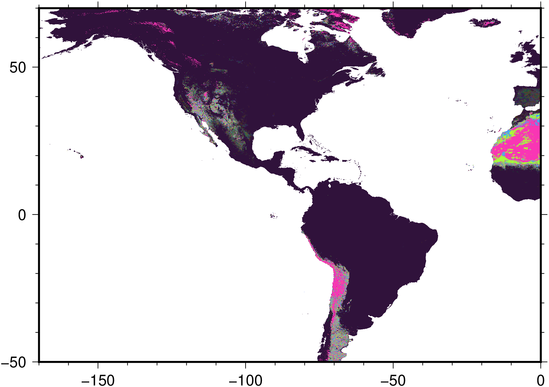
@KristofKoch I don’t know if you are still pursuing this but I used as a test to the new capabilities of the Julia wrapper (stronger GDAL integration). “average” is not a good filter because the data is categorical but GDAL also has a “most frequent” operator that looks good for this purpose. The whole process seemed to have used ~1.75 GB of RAM.
fname = "PROBAV_LC100_global_v3.0.1_2019-nrt_Bare-CoverFraction-layer_EPSG-4326.tif";
tic(); I = gdaltranslate(fname, R="-170/0/-50/70", I=0.05, ["-r", "mode"]);toc()
elapsed time: 73.1168982 seconds
Now, oddly the original does not come with a color table and the site does not provide anyone and mention 23 classes, which is strange because that’s not what is in the file. I see values up to 100, so made a quick dummy cpt and used it. The result is only half-convincing.
C = makecpt(range=(1,100));
image_cpt!(I, C)  # Add the colormap to the image because grdimage does not allow to do it
imshow(I, fmt=:png)